Preliminary Info
This tutorial series assumes you are already knowledgeable in basic quantum mechanics (state vectors/wave functions), statistics, linear algebra, and Python.
This series is for those who want to focus on directly learning IBM Qiskit, the Python library. To learn Qiskit along with the necessary math, visit IBM Quantum Learning.
Once the necessary Qiskit concepts are introduced, we will delve directly into quantum computing theory, where chapters will become more math-intensive.
If you do not know the math yet, do not use this tutorial. Understanding the math is essential for understanding how the code works.
I provide chapters covering the same rough topics as IBM’s textbook, with exercises at the end. To fully master Qiskit, it is important to experiment with Qiskit yourself at the end of each chapter to get a better grasp before starting the next one.
For any typos, issues, or suggestions on this tutorial, please fork the website repo (.md files under /content/qiskit/), or email me. Thanks!
$$ \sim * \backsim $$
Table of Contents
- § 1. States, Measurements, & Operations
- § 2. Single Qubit Quantum Gates
- § 3. Quantum Gates Review
- Exercises
- Solutions
$$ \backsim * \sim $$
To begin learning Qiskit, the software used to work with quantum circuits, we need to understand how to define and work with qubits.
§ 1. States, Measurements, & Operations
Defining Qubit Statevectors
The Statevector class provides functionality for defining and manipulating
quantum statevectors (or wave functions, if you are a physicist like me).
Below I import the Statevector class from qiskit.quantum_info and generate three statevectors u, vand w.
from qiskit.quantum_info import Statevector
import numpy as np
from numpy import sqrt

u = Statevector([1/sqrt(2), 1/sqrt(2)])
v = Statevector([(1 + 2.0j)/3, -2/3])
w = Statevector([1/3, 2/3])
The Statevector class also provides a draw() method for displaying statevectors in $\LaTeX$ format (or just plain text if you prepfer).
display(u.draw('latex'))
display(v.draw('latex'))

The Statevector() class uses the computational basis by default: {${|0\rangle, |1\rangle}$}. We can check if these statevectors are valid using the is_valid() method.
print(f"Statevector u is valid? {u.is_valid()}")
print(f"Statevector w is valid? {w.is_valid()}")

A valid statevector is one who’s Euclidean norm equals 1. The norm of all the coefficients squared must equate to 1.
Simulating Measurements
Using the measure() method is one way to measure statevectors in Qiskit.
# creating qubit wave function & displaying it
v = Statevector([(1 + 2.0j)/3, -2/3])
display(v.draw("latex"))

# measuring
v.measure()
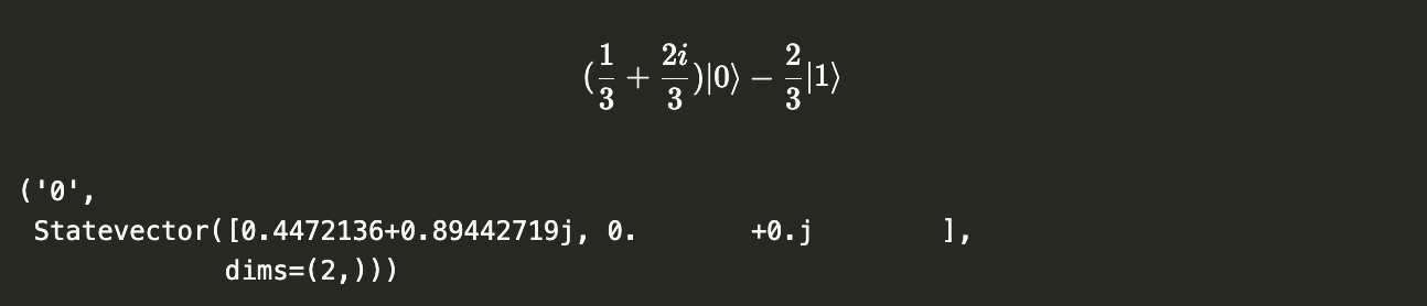
Since the result of measurements is probabilistic, measuring the above statevector could yield different results.
Upon measurement, the qubit collapses into either $|0\rangle$ or $|1\rangle$, since we have been using the computational basis {${ |0\rangle, |1\rangle }$} to define our statevectors so far.
v.measure() returns a tuple which stores information on the eigenvalue measured, the collapsed wave function, and the dimension of the wave function.
v.measure()[0] # measured eigenvalue
v.measure()[1] # collapsed resultant wave function
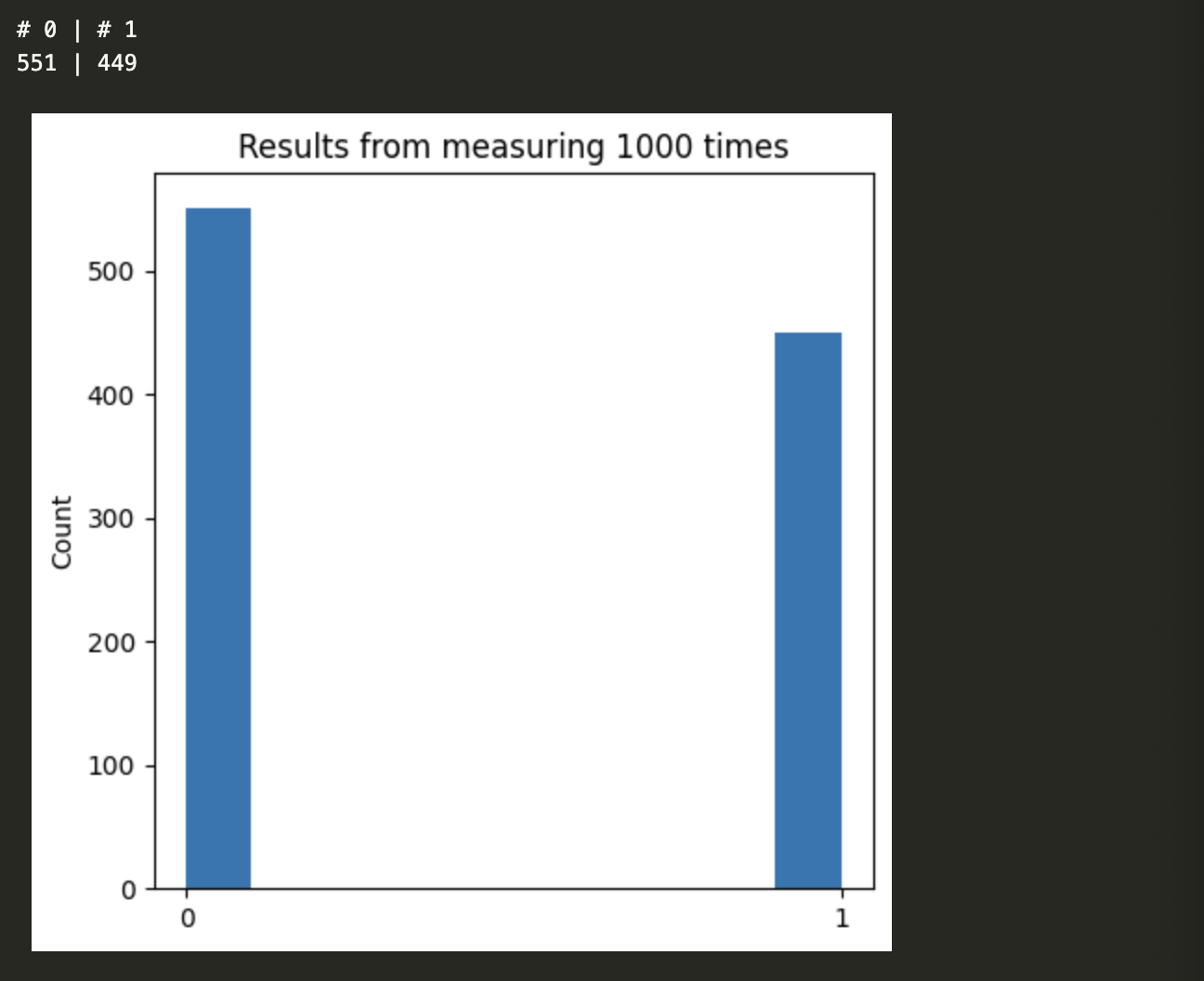
If we run many iterations of v.measure() we should get a graph that approximates the intrinsic probabilities of each component.
import matplotlib.pyplot as plt

results = np.empty([0])

num_runs = 1000

for i in range(num_runs):
    results = np.append(results, v.measure()[0]) # storing resulting eigenvalues

num_0 = len(np.where(results == '0')[0]) # # measurements yielding 0
num_1 = len(np.where(results == '1')[0]) # # measurements yielding 1

fig, axis = plt.subplots(1, 1, figsize = (5, 5))
plt.hist(results)
plt.title(f"Results from measuring {num_runs} times")
plt.ylabel("Count")

print("{:>3} | {:>3}".format("# 0", "# 1"))
print("{:>3} | {:>3}".format(num_0, num_1))
Qiskit provides a simpler and more direct way to visualize probabilities using the plot_histogram() method in qiskit.visualization.
from qiskit.visualization import plot_histogram

statistics = v.sample_counts(1000) # directly make 1000 measurements
                                   # and store results in `statistics`
print(statistics)
plot_histogram(statistics, figsize = (5, 5)) # makes histogram directly
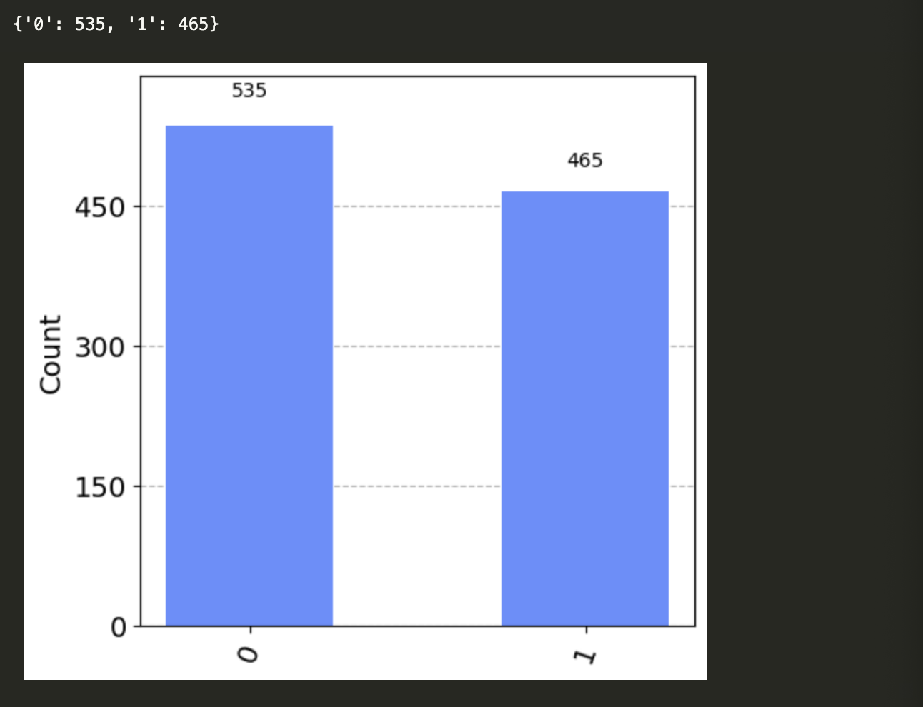
We see the results are almost identical. If we took an infinite number of measurements and collected all the results, the probabilities would match what is predicted by the statevector.
By now you should start to feel that Qiskit is just plain and simple python. While Qiskit is indeed a Python library, it may seem like a whole new language to many. One just has to understand how to work with all the features of Qiskit within Python. The first step is understanding all the quantum gates/operators.
§ 2. Single Qubit Quantum Gates
We start with the Pauli Operators, used to measure the spins of elementary particles. Spin is one way to define qubits in real life (spin up $|\uparrow\rangle$ represents $|0\rangle$, and spin down $|\downarrow\rangle$ represents $|1\rangle$).
- Pauli $X$ (NOT) Operator
The simplest logic gate is the Pauli-$X$ or NOT operator. It inverts the value of a qubit from $0 \rightarrow 1$ or $1 \rightarrow 0$ in the computational basis. Its matrix representation is:
 Figure 1: Pauli $X$ Gate
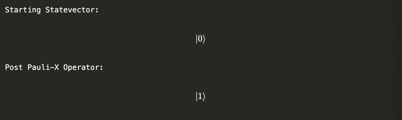
We can see its effect on the statevector $|0\rangle = v= \left(1 \atop 0\right)$
from qiskit.quantum_info import Operator

X = Operator([[0, 1], [1, 0]]) # Pauli X Operator

v_initial = Statevector([1, 0]) # Statevector

print("Starting Statevector:")
display(v_initial.draw("latex"))

v_final = v_initial.evolve(X) # applies X on v_i

print("Post Pauli-X Operator:")
display(v_final.draw("latex"))
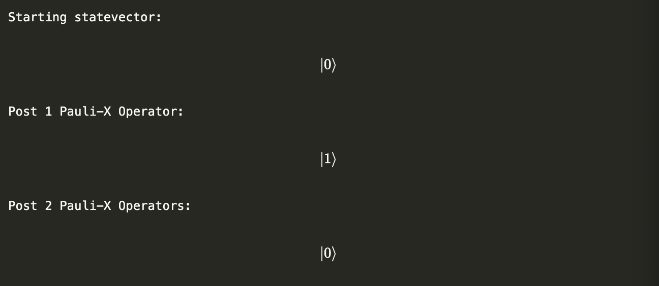
If we apply two $X$-gates in succession, the qubit flips back to its original state $|0\rangle$.
v_intermediate = v_initial.evolve(X)
v_final = v_intermediate.evolve(X)

print("Starting statevector:")
display(v_initial.draw("latex"))

print("Post 1 Pauli-X Operator:")
display(v_intermediate.draw("latex"))

print("Post 2 Pauli-X Operators:")
display(v_final.draw("latex"))
Next, let’s introduce the other 2 Pauli Operators (besides the identity matrix).
- Pauli $Y$ Operator
 Figure 2: Pauli $Y$ Gate
- Pauli $Z$ Operator
 Figure 3: Pauli $Z$ Gate
The $Z$ gate performs a “phase-flip” operation: $$ Z|0\rangle = |0\rangle \qquad Z|1\rangle = -|1\rangle $$
The $Y$ gate performs both a bit-flip and a phase-flip. Phase operations are described by the matrix

(i.e., they leave the $|0\rangle$ constant and add a phase to the $|1\rangle$ component). The $Z$ operator is the case of $P_\pi$.
Other important operators include:
- Hadamard Operator
 Figure 4: Hadamard Gate
The Hadamard Gates puts the standard basis states {\( |0\rangle, |1\rangle \)} into a superposition.

Applying the same operations to $|+\rangle$ and $|-\rangle$,
$$ H|+\rangle = |0\rangle $$ $$ H|-\rangle = |1\rangle $$
Since $|+\rangle$ and $|-\rangle$ have the same probability distributions for measuring 0 or 1, measuring either provides no information about the initial state. By applying the $H$ gate, we obtain 0 if the initial state was $|+\rangle$ and 1 if it was $|-\rangle$.
- T Operator
The T gate is equivalent to a $P_{\pi/4}$ phase operation.
 Figure 5: T Gate
§ 3. Quantum Gates Review
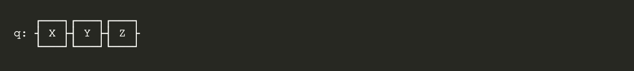
Let’s define a quantum circuit using qiskit.QuantumCircuit() and implement
some gates on $|0\rangle$. We will fully discuss the QuantumCircuit() method in chapter 3.
from qiskit import QuantumCircuit

circuit = QuantumCircuit(1) # initialize circuit with 1 qubit

circuit.x(0)
circuit.y(0)
circuit.z(0)

circuit.draw()
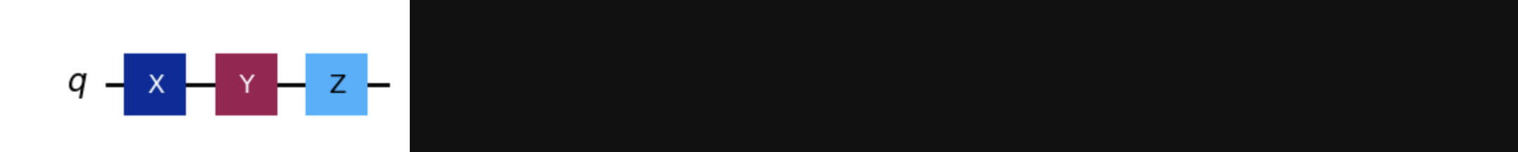
You can also display the circuit more colorfully using the output = 'mpl' parameter:
circuit.draw('mpl')
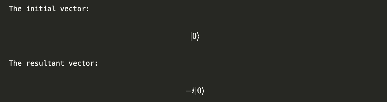
ket0 = Statevector([1, 0])

v = ket0.evolve(circuit) # Apply the circuit above on the |0> statevector
                         # Note the operations are applied sequentially
                         # left-to-right

print("The initial vector:")
display(ket0.draw("latex"))

print("The resultant vector:")
display(v.draw("latex"))
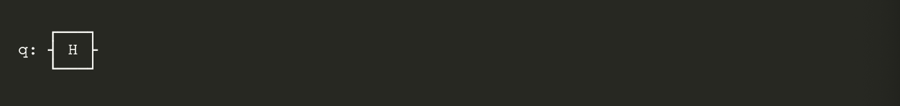
Let’s apply the Hadamard Gate $H$ on $|0\rangle$.
For the following code segments, predict what the output will be based on information provided about the gates.
circuit = QuantumCircuit(1)

circuit.h(0)
circuit.draw()
v = ket0.evolve(circuit)
v.draw("latex")

Applying the Hadamard Gate on v = $|+\rangle$ (the same as applying two Hadamard Gates on ket0 = $|0\rangle$:
w = v.evolve(circuit) # Applying the same circuit on v
                      # (a second hadamard gate on |0>)
w.draw("latex")

We get back the original statevector $|0\rangle$.
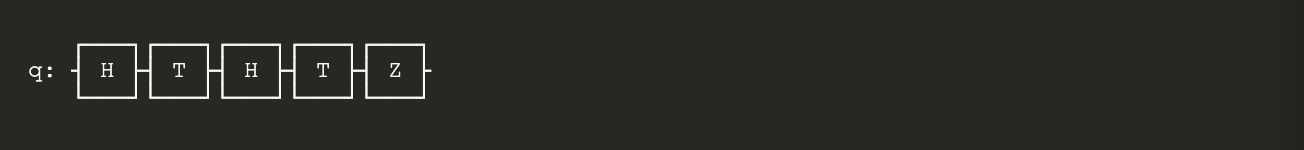
Now let’s build a random circuit with a bunch of gates and apply it on $|0\rangle$.
circuit = QuantumCircuit(1)

circuit.h(0)
circuit.t(0)
circuit.h(0)
circuit.t(0)
circuit.z(0)

circuit.draw()
ket0 = Statevector([1, 0])
v = ket0.evolve(circuit)

v.draw("latex")

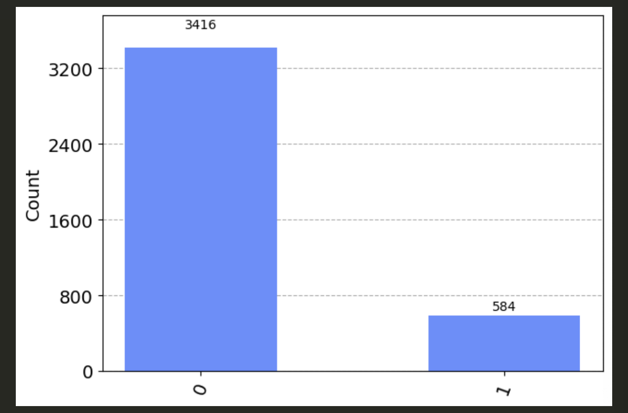
We get a complex statevector. Let’s check its probability distribution
statistics = v.sample_counts(4000)
plot_histogram(statistics)
Exercises
Plot the probability distribution from measuring the $|+\rangle$ and $|-\rangle$ statevectors.
Perform a Hadamard Gate on $|0\rangle$ twice. What is the final statevector?
Perform a Phase $P_\frac{\pi}{3}$ operation on $|1\rangle$. What is the final statevector?
$\hspace{1px}$
$\hspace{1px}$
$\hspace{1px}$
$\hspace{1px}$
$\hspace{1px}$
$\hspace{1px}$
Solutions
First attempt the problems!
Problem 1.
from qiskit.quantum_info import Statevector
from qiskit import QuantumCircuit
# We can generate the plus and minus vectors via two different ways.
# 1. Implementing an H gate on the |0> and |1> vectors, respectively
# 2. Calling directly from Statevector.from_label("+") and .from_label("-")
# Method 1 ---------------
ket0 = Statevector([1, 0]) # We could also say ket0 = Statevector.from_label("0")
ket1 = Statevector([0, 1])
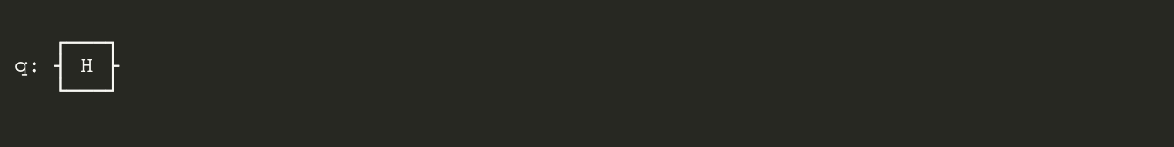
circuit_with_a_hadamard_gate = QuantumCircuit(1)
circuit_with_a_hadamard_gate.h(0)
circuit_with_a_hadamard_gate.draw()
plus = ket0.evolve(circuit_with_a_hadamard_gate)
minus = ket1.evolve(circuit_with_a_hadamard_gate)

display(plus.draw("latex"))
display(minus.draw("latex"))

# Method 2 -----------------------
plus = Statevector.from_label("+")
minus = Statevector.from_label("-")

display(plus.draw("latex"))
display(minus.draw("latex"))

from qiskit.visualization import plot_histogram

plus_stats = plus.sample_counts(1000)
minus_stats = minus.sample_counts(1000)

print("|+>")
display(plot_histogram(plus_stats))

print("|->")
display(plot_histogram(minus_stats))
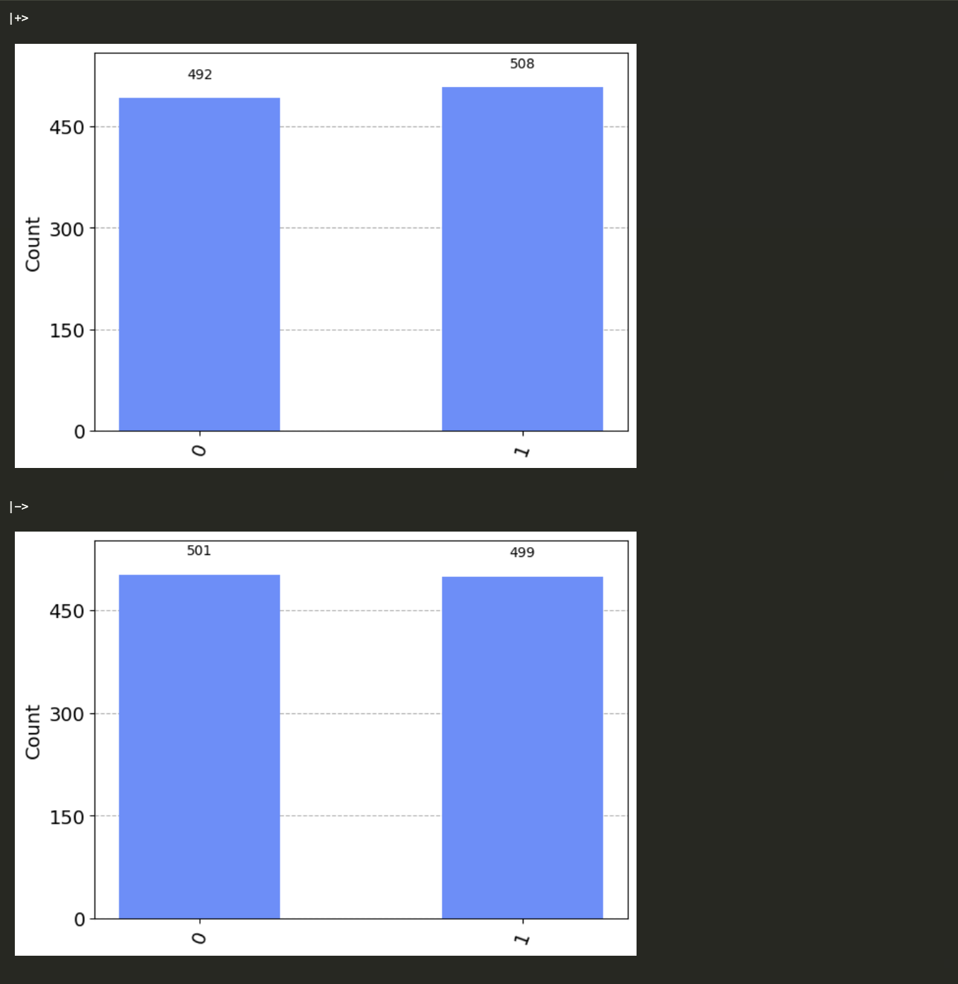
We see the probabilities for measuring 0 and 1 are roughly equal for both $|+\rangle$ and $|-\rangle$ – as they should be.
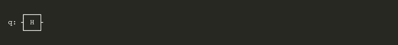
Problem 2.
Let’s define a QuantumCircuit with one Hadamard Gate. This way we do not
have to define the Hadamard matrix with the Operator() method.
from qiskit.quantum_info import Statevector
from qiskit import QuantumCircuit

circuit = QuantumCircuit(1)

circuit.h(0)

circuit.draw()
ket0 = Statevector([1, 0]) # or you could call ket0 = Statevector.from_label("0")
ket0.draw('latex')

Let’s implement the circuit once (one Hadamard gate) on $|0\rangle$ and see the result.
display(ket0.evolve(circuit).draw("latex"))

We get the $|+\rangle$ as expected. Now let’s run this new statevector back through the circuit. (This is the same as applying a Hadamard gate twice on $|0\rangle$).
plus = ket0.evolve(circuit)

display(plus.evolve(circuit).draw("latex"))

We see that applying two Hadamard gates to the $|0\rangle$ statevector re-yields $|0\rangle$.
Problem 3.
Recall that a Phase operation is given by

Therefore, $P_{\pi/3}$

Let’s define this operator in Qiskit and see its effect on $|1\rangle$.
from qiskit.quantum_info import Operator
import math

ket1 = Statevector([0, 1]) # or you could call Statevector.from_label("1")
PhasePi3 = Operator([[1, 0], [0, math.cos(math.pi / 3) + 1j * math.sin(math.pi / 3)]]) # using Euler's formula

display(ket1.evolve(PhasePi3).draw("latex"))