$$ \sim * \backsim $$
Table of Contents
$$ \backsim * \sim $$
§ 4. Multi-Qubit Quantum Gates
Now that we understand single-qubit gates, let’s explore multi-qubit operators, which act on more than one qubit / statevector.
A multi-qubit state $$|XY\rangle$$ is the tensor product of two single-qubit states:
$$ |XY\rangle = |X\rangle \otimes |Y\rangle = |X\rangle|Y\rangle$$
Let’s discuss some crucial Quantum Gates that operaton on multi-qubit states.
- SWAP Gate
The SWAP gate exchanges the states of two qubits:
$$ \text{SWAP} |a\rangle |b\rangle = |b\rangle |a\rangle $$
Its matrix representation is shown below
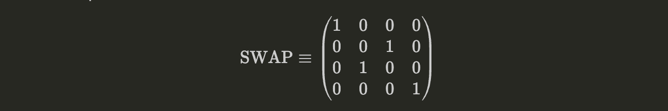 Figure 6: SWAP Gate
Controlled Operations
A controlled $U$ operator performs an action on a target qubit based on the state of a control qubit.
For qubits defined in the computational basis states $|0\rangle$ and $|1\rangle$, a controlled $U$ operation can be represented as:
$$ CU = |0\rangle \langle 0| \otimes I_R + |1\rangle\langle 1| \otimes U $$
To illustrate this, let’s discuss the Controlled NOT (CNOT) gate.
- CX / CNOT Gate
The CNOT gate flips the target qubit if the control qubit is in state $|1\rangle$, and leaves the target qubit unchanged if the control qubit is in state $|0\rangle$.
The action of a CNOT gate is depicted as:
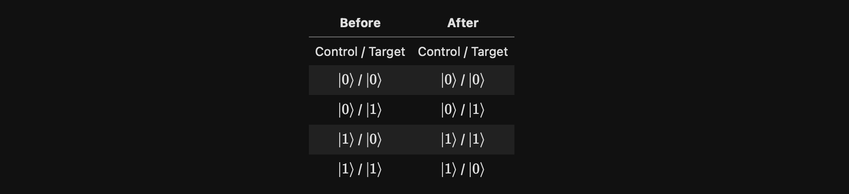
It leaves the control qubit unchanged regardless. Its matrix representation is:
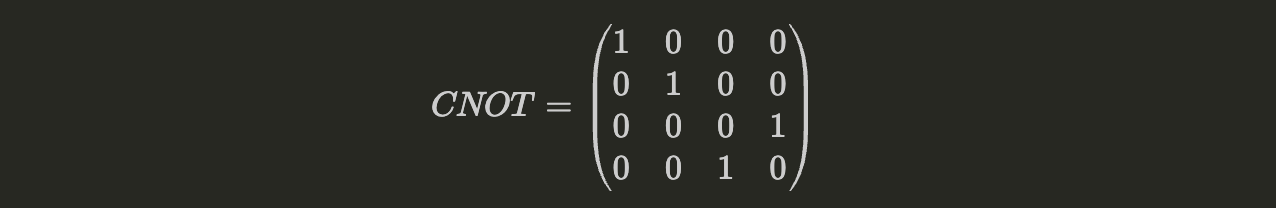 Figure 7: CNOT Gate
Controlled operations can be performed on both single and multi-qubit states. The control or target can be a system of qubits. For example, the CCNOT (controlled-controlled NOT) gate, also known as the Toffoli Gate, is a CNOT gate with 2 control qubits and 1 target qubit. The target qubit gets inverted if and only if both control qubits are in state $|1\rangle$.
Now, let’s discuss how to generate multi-qubit states. We have already learned how to generate single-qubit states using the Statevector() class in the previous chapter. To generate a multi-qubit state, we need to understand how to perform tensor products.
§ 5. Tensor Products
First, let’s create the multi-qubit statevector $|01\rangle$ as a tensor product of $|0\rangle \otimes |1\rangle$:
zero, one = Statevector.from_label("0"), Statevector.from_label("1")
zero.tensor(one).draw("latex")

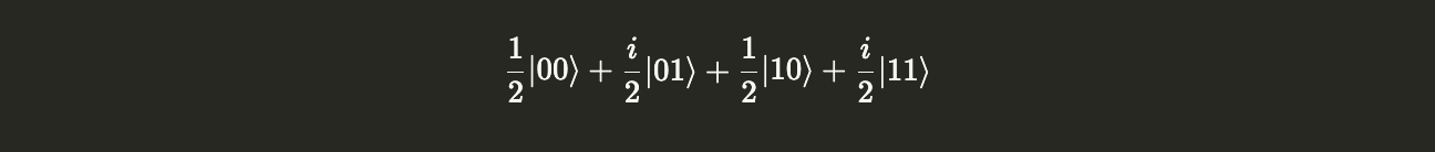
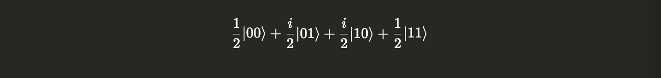
Next, let’s create the statevectors $|+\rangle$ and $\frac{1}{\sqrt{2}}(|0\rangle + i|1\rangle)$, and combine them to form a new statevector $|\psi\rangle$:
plus = Statevector.from_label("+")
i_state = Statevector([1/sqrt(2), 1j/sqrt(2)])

psi = plus.tensor(i_state)
psi.draw("latex")
We can also take the tensor product of operators. The tensor product $C$ of the operators $X$ and $Y$, where $C = X \otimes Y$, can act simultaneously on a 2-qubit system. This is equivalent to applying $X$ to the first qubit and $Y$ to the second qubit, and then taking the tensor product.
To illustrate this, consider the following circuit:
circuit = QuantumCircuit(2)

circuit.x(0)
circuit.y(1)
display(circuit.draw())
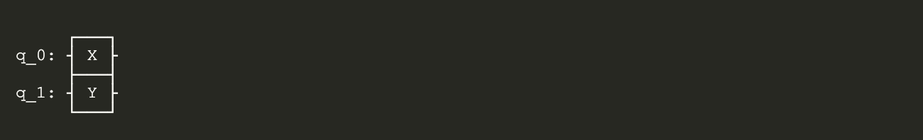
This is the same as applying the $C = X \otimes Y$ gate on the tensor product $q_0 \otimes q_1$.
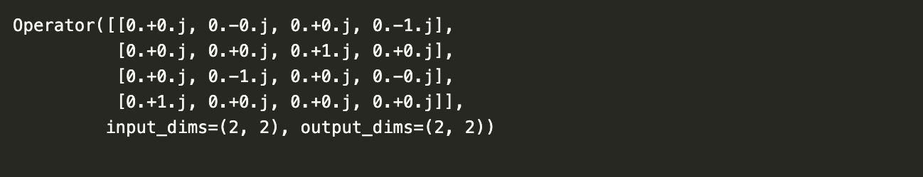
We can generate tensor products between operators in the same way as with statevectors:
X = Operator([[0, 1], [1, 0]])
Y = Operator([[0, -1j], [1j, 0]])

C = X.tensor(Y)
print(C)
Let’s show that applying $X$ on qubit $|0\rangle$ and $Y$ on qubit $|1\rangle$ and then taking the resulting tensor product, is the same as applying $C = X \otimes Y$ to $|01\rangle = |0\rangle \otimes |1\rangle$.
ket0 = Statevector([1, 0])
ket1 = Statevector([0, 1])
ket_combined = ket0.tensor(ket1)

# individually applying X and Y to |0> and |1> separately
ket0f = ket0.evolve(X)
ket1f = ket1.evolve(Y)
ket_combinedf = ket0f.tensor(ket1f)

print("X|0> ⊗ Y|1> ")
display(ket_combinedf.draw("latex"))

# applying combined operator to both,
# redefining ket_combinedf using ket_combined
ket_combinedf = ket_combined.evolve(X ^ Y) # X ^ Y = X ⊗ Y = C

print("(X ⊗ Y)|01>")
display(ket_combinedf.draw("latex"))
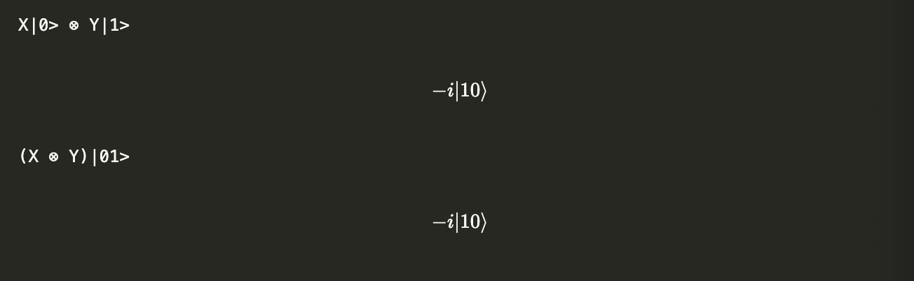
They’re the same! Let’s go back to the $|\psi\rangle$ vector we defined earlier,
psi.draw("latex")
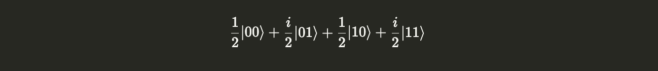
Now, let’s create a CNOT operator and calculate $CNOT|\psi\rangle$.
CX = Operator(
    [
        [1, 0, 0, 0],
        [0, 1, 0, 0],
        [0, 0, 0, 1],
        [0, 0, 1, 0],
    ]
)

psi.evolve(CX).draw("latex")
Compare the coefficients of the $|10\rangle$ and $|11\rangle$ states.
Now that we understand how to implement operators on multi-qubit states, let’s move on to implementing partial measurements on individual qubits of a multi-qubit state.
§ 6. Partial Measurements
In the previous chapter, we used the measure() method to simulate a measurement of a quantum statevector. This method returned the measured qubit value, and the resultant collapsed statevector post-measurement.
By default, `measure()`` measures all qubits in the statevector. However, we can provide a list of integers to measure only the qubits at those indices.
The following example demonstrates how to create and partially measure a specific state. We will create the state
$$ W = \frac{1}{\sqrt{3}} ( |001\rangle + |010\rangle + |100\rangle). $$
using the Statevector() class:
W = Statevector([0, 1, 1, 0, 1, 0, 0, 0] / sqrt(3))
W.draw("latex")

To understand how the above state was generated using Statevector(), note that each parameter index (0 or 1) represents a possible 3-qubit state:
- $|000\rangle$ (index 0)
- $|001\rangle$ (index 1)
- $|010\rangle$ (index 2)
- $|011\rangle$ (index 3)
- $|100\rangle$ (index 4)
- $|101\rangle$ (index 5)
- $|110\rangle$ (index 6)
- $|111\rangle$ (index 7)
The statevector $W$ has a value of 1 at indices 1, 2, and 4, indicating the presence of the states $|001\rangle$, $|010\rangle$, and $|100\rangle$.
Let’s simulate a measurement on the rightmost qubit (which has index 0). Note that this is the opposite of the usual convention, where qubit indices start from the right.
result, new_statevector = W.measure([0]) # measure qubit 0

print(f"Measured: {result}\nState after measurement:")
new_statevector.draw("latex")
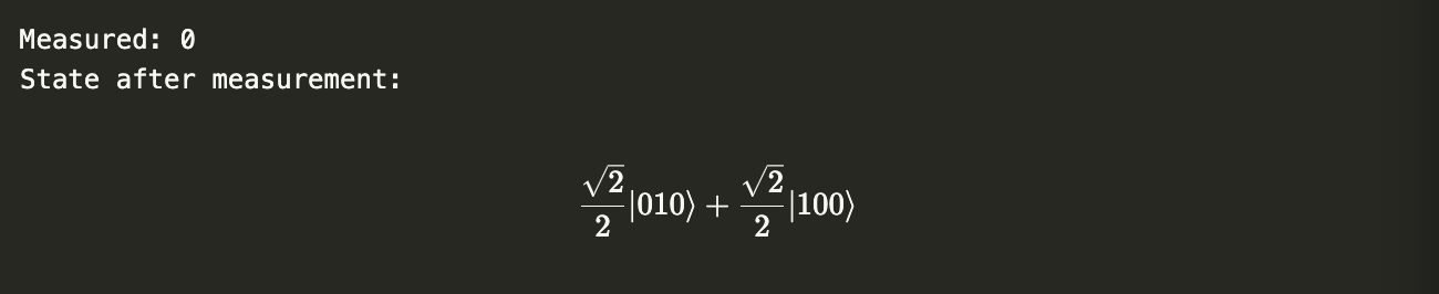
Run the above cell multiple times to observe different results. Notice the following:
- Measuring a
1means both the other qubits are $|0\rangle$ - Meausring a
0leaves the remaining two qubits in the state $$\frac{1}{\sqrt{2}}(|01\rangle + |10\rangle).
In the next chapter, we will explore `QuantumCircuit()``, which allows us to fully manipulate and work with any $n$-qubit state. Before moving on, try the following exercises to ensure you understand how to generate and measure multi-qubit states.
Exercises
Generate the tensor product $|+\rangle |-\rangle$ and implement a CNOT gate on the result. The CNOT gate should have the first, left-most qubit as the control.
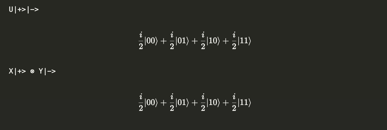
Generate the tensor product operator $U$ between the Pauli-$X$ and Pauli-$Y$ operators ($U = X \otimes Y$). Show that applying $U |+\rangle |-\rangle$ yields the same result as $X|+\rangle \otimes Y|-\rangle$.
$\hspace{1px}$
$\hspace{1px}$
$\hspace{1px}$
$\hspace{1px}$
$\hspace{1px}$
$\hspace{1px}$
Solutions
Problem 1.
Let’s first generate the $|+\rangle |-\rangle$ statevector.
from qiskit.quantum_info import Statevector, Operator

plus = Statevector.from_label("+")
minus = Statevector.from_label("-")

plusminus = plus.tensor(minus) # Generating |+>|->
plusminus.draw('latex')

Let’s build the CNOT matrix and apply it on $|+\rangle |-\rangle$.
CNOT = Operator(
    [
        [1, 0, 0, 0],
        [0, 1, 0, 0],
        [0, 0, 0, 1],
        [0, 0, 1, 0]
    ]
)

plusminus.evolve(CNOT).draw("latex")

We see that the coefficients in front of the $|10\rangle$ and $|11\rangle$ switched. (The $|11\rangle$ state became $|10\rangle$ and vice versa).
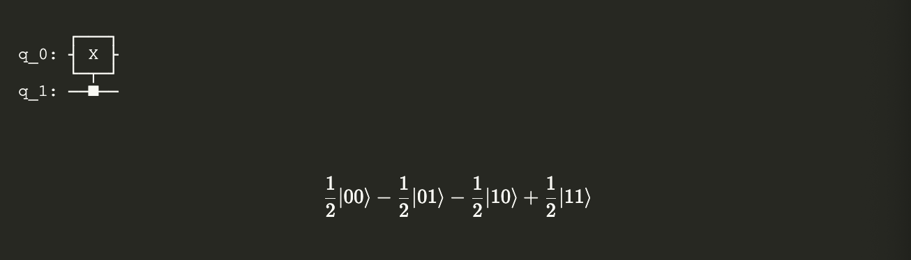
I present a second method using qiskit.QuantumCircuit(). We have not fully discussed QuantumCircuit yet, so consider this a sneak peek.
from qiskit import QuantumCircuit # We have not done fully introduced QuantumCircuits yet
                                  # You can consider this a sneak-peek

circuit = QuantumCircuit(2)

circuit.cx(1, 0) # CNOT gate with the left-most (index 1) qubit as the control

display(circuit.draw())

plusminus = Statevector.from_label("+").tensor(Statevector.from_label("-")) # Generating |+>|->
plusminus.evolve(circuit).draw('latex')
Problem 2.
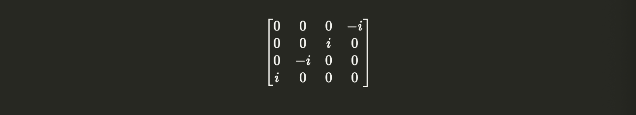
Let’s first create the Pauli-$X$ and Pauli-$Y$ operators as well as the operator $U = X\otimes Y.$
from qiskit.quantum_info import Operator

X = Operator(
    [
        [0, 1],
        [1, 0]
    ]
)

Y = Operator(
    [
        [0, -1j],
        [1j, 0]
    ]
)

U = X.tensor(Y)
U.draw("latex")
Now let’s generate the $|+\rangle$ and $|-\rangle$ states, along with their tensor product $|+\rangle |-\rangle$ and get the results of each operation from the question.
plus = Statevector.from_label('+')
minus = Statevector.from_label('-')

plusminus = plus.tensor(minus)


#Implementing U|+>|->
print("U|+>|->")
display(plusminus.evolve(U).draw('latex'))

# Implementing X|+> ⊗ Y|->
print("X|+> ⊗ Y|->")
display(plus.evolve(X).tensor(minus.evolve(Y)).draw('latex'))
Previous – Single-Qubit States $\sim$*$\backsim$ Next – Quantum Circuits