$$ \sim * \backsim $$
Table of Contents
$$ \backsim * \sim $$
So far, we’ve discussed working with single-qubit and multi-qubit states. We’ve also covered various operators and used the .evolve() method to apply these operators to statevectors.
Now it’s time to start building our own Quantum Circuits. These circuits allow us to visualize the change of information and trace the evolution of qubits through a series of quantum gates.
First, let’s the essential tools for working with quantum circuits:
from qiskit import QuantumCircuit, QuantumRegister, ClassicalRegister
from qiskit.primitives import Sampler
from qiskit.visualization import plot_histogram
§ 7. Building Quantum Circuits
We build a circuit using the QuantumCircuit() method.
circuit = QuantumCircuit(1) # Quantum Circuit with 1 Qubit

circuit.h(0) # Apply a Hadamard Gate
circuit.s(0) # Apply an S Gate
circuit.h(0) # Apply another Hadamard Gate
circuit.t(0) # Apply a T gate

display(circuit.draw()) # Gates are performed left-to-right

By default, the QuantumCircuit() method initializes every qubit to the $|0\rangle$ state.
In Qiskit, the topmost qubit in a circuit diagram has index 0 and corresponds to the rightmost position in a tuple of qubits. Qiskit’s default names for the qubits in an $n$-qubit circuit are represented by the $n$-tuple $(q_{n-1}, \cdots, q_0)$, with $q_0$ being the qubit on top and $q_{n-1}$ on the bottom in quantum circuit diagrams.
We can also create a 2-qubit gate as follows:
# Generating Identical 2-qubit circuits
# circuit_default has default q_0, q_1 names
# circuit_named allows us to define the names of the qubit using `QuantumRegister()`

circuit_default = QuantumCircuit(2) # 2 Qubits

circuit_default.h(0) # Hadamard Gate on the topmost qubit
circuit_default.cx(0, 1) # CNOT gate (control, target)

display(circuit_default.draw())

#-----------------------------#

X = QuantumRegister(1, "X")
Y = QuantumRegister(1, "Y")

circuit_named = QuantumCircuit(X, Y)

circuit_named.h(X)
circuit_named.cx(X, Y)

display(circuit_named.draw())

We have created two identical circuits, one with default names and the other with custom names. Both circuits contain a Hadamard Gate on the first qubit and a CNOT gate with the first qubit as the control and the second as the target.
Let’s see the action of the above circuit on the standard computational basis states for a 2-qubit system:
$$|00\rangle \quad |01\rangle \quad |10\rangle \quad |11\rangle$$
zero = Statevector.from_label("0")
one = Statevector.from_label("1")

standard_basis_states = [zero.tensor(zero), zero.tensor(one),
                         one.tensor(zero), one.tensor(one)]

names = ["|00>", "|01>", "|10>", "|11>"]

for i in range(len(standard_basis_states)):
    print(f"{names[i]} -->")
    display(standard_basis_states[i].evolve(circuit_named).draw("latex"))
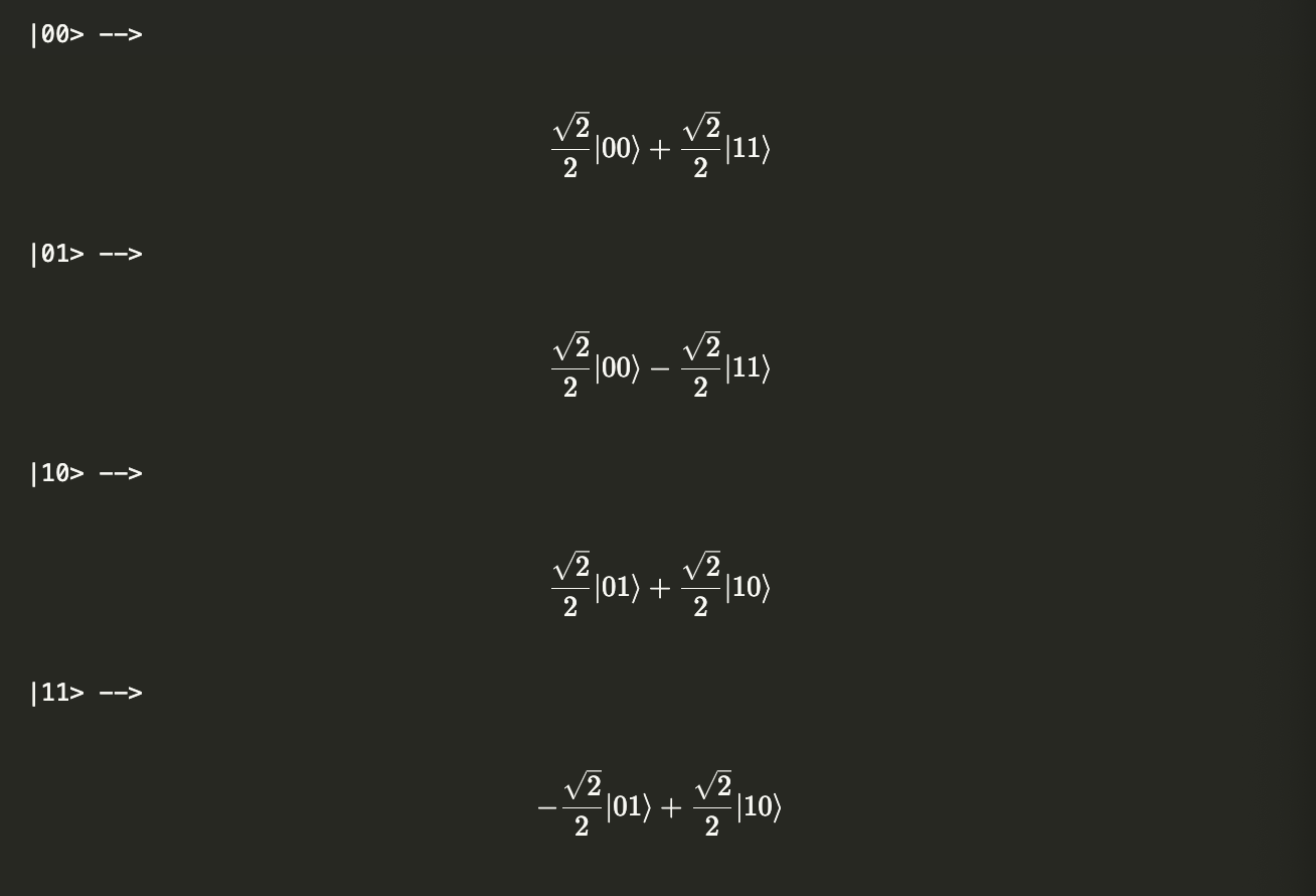
The circuit above generates the Bell states (entangled states that form a basis):
$$|\phi^+\rangle = \frac{1}{\sqrt{2}}|00\rangle + \frac{1}{\sqrt{2}}|11\rangle $$ $$|\phi^-\rangle = \frac{1}{\sqrt{2}}|00\rangle - \frac{1}{\sqrt{2}}|11\rangle $$ $$|\psi^+\rangle = \frac{1}{\sqrt{2}}|01\rangle + \frac{1}{\sqrt{2}}|10\rangle $$ $$|\psi^-\rangle = \frac{1}{\sqrt{2}}|01\rangle - \frac{1}{\sqrt{2}}|10\rangle $$
except the final $|11\rangle$ state becomes the negative of the fourth $|\psi^-\rangle$ Bell state.
This circuit provides a way to convert the standard computational basis into the Bell Basis. To eliminate the -1 phase factor on the last state ($-|\psi^-\rangle$), we can add a controlled-$Z$ gate at the beginning.
circuit = QuantumCircuit(2)

circuit.cz(0, 1)
circuit.h(0)
circuit.cx(0, 1)

circuit.draw()

Implementing the above altered circuit on the standard computational basis states:
for i in range(len(standard_basis_states)):
    print(f"{names[i]} --> ")
    display(standard_basis_states[i].evolve(circuit).draw("latex"))
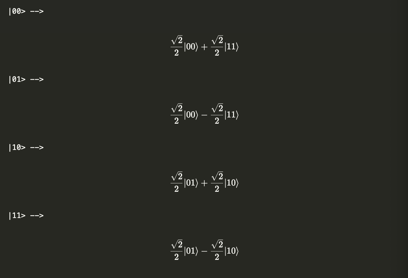
This results in the Bell Basis.
Classical Bits
Quantum circuits can contain any number of qubit wires and may also include classical bit wires, indicated by double lines:
X = QuantumRegister(1, "X")
Y = QuantumRegister(1, "Y")
A = ClassicalRegister(1, "A")
B = ClassicalRegister(1, "B") # Using `Classical Register` to customize the name
                              # for two separate classical bits

circuit = QuantumCircuit(X, Y, A, B)
circuit.h(X)
circuit.cx(X, Y)
circuit.measure(X, A)
circuit.measure(Y, B)

circuit.draw()

The measurement gates represent standard basis measurements, resulting in either $|0\rangle$ or $|1\rangle$ as the eigenvectors/post-measurement states. The measurement gate changes the qubits into their post-measurement states, while the classical measurement outcomes (0 for $|0\rangle$ or 1 for $|1\rangle$) are overwritten onto the classical bits to which the arrows point.
Sampler Primitive
A primitive is the smallest processing instruction for a certain level of abstraction. It allows a user to write quantum algorithms without having to worry about hardware details.
The Sampler() primitive calculates probabilities of bitstrings outputted from quantum circuits.
The above circuit can be simulated using the Sampler() primitive.
sampler = Sampler() # Initialize Sampler
job = sampler.run(circuit)
results = job.result()

statistics = results.quasi_dists[0].binary_probabilities()
plot_histogram(statistics)
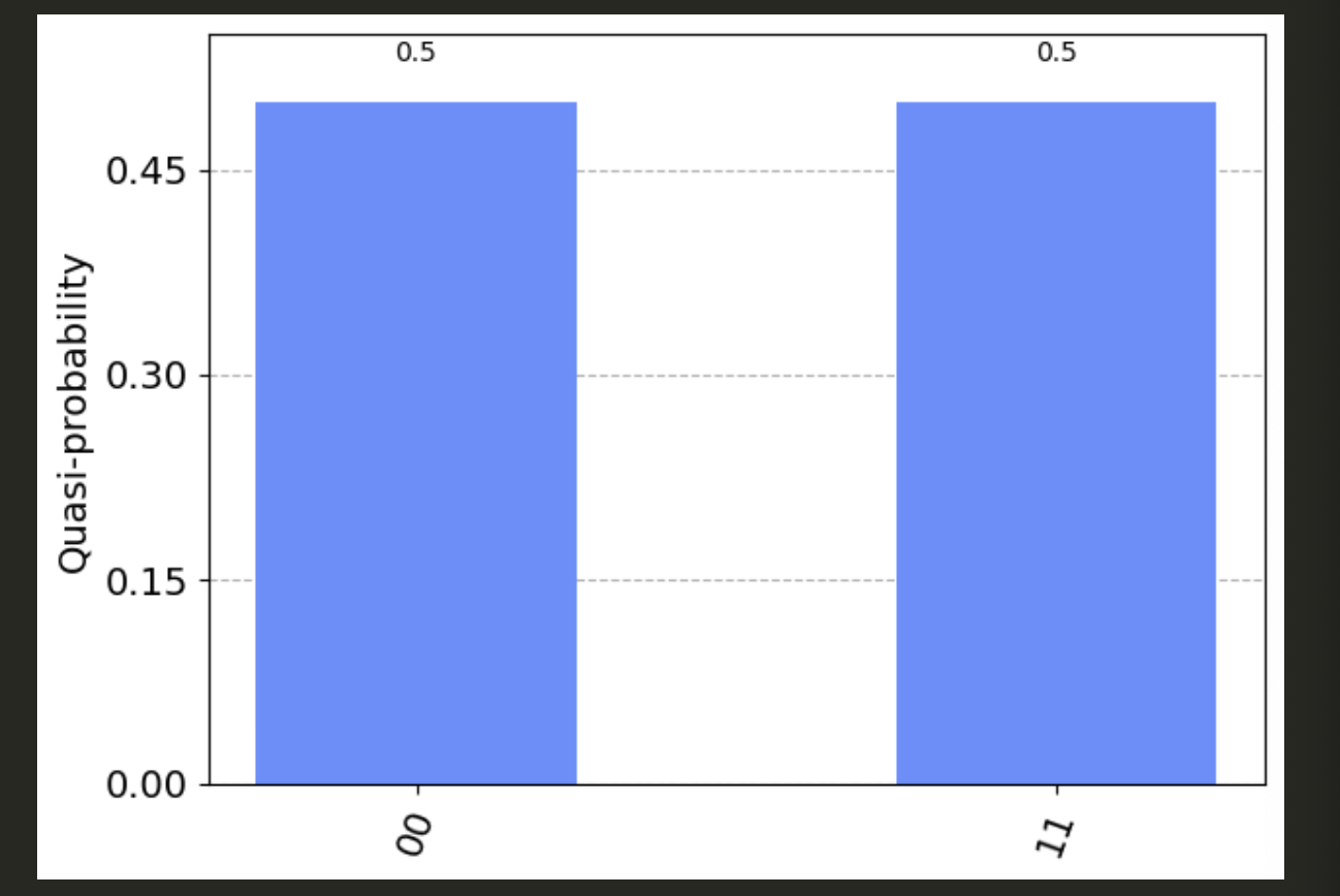
We use the primitive by calling its run() method with the circuit. If the run(shots = ) parameter is unspecified, it returns the exact probabilities.
Calling the result() method afterwards provides output samples and corresponding metadata.
The main takeaway is that the results show an equal probability for the measurement yielding the classical values of 00 and 11.
§ 8. Quantum Circuits Review
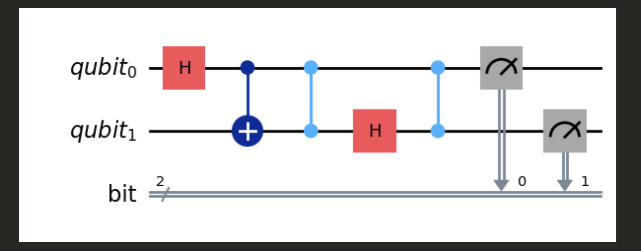
Let’s experiment with a complex quantum circuit, involving both qubits and classical bits, and observe the resultant probabilities.
q = QuantumRegister(2, name = 'qubit')
c = ClassicalRegister(2, name = 'bit')

circuit = QuantumCircuit(q, c)

circuit.h(q[0])
circuit.cx(q[0], q[1])      # Note you do not have to specify q[...]
circuit.cz(q[1], q[0])      # I just do it for readability
circuit.h(q[1])
circuit.cz(q[0], q[1])
circuit.measure(q, c)

circuit.draw('mpl')
sampler = Sampler() # sampler initialization

job = sampler.run(circuit, shots = 128) # sampling 128 runs
results = job.result()

statistics = results.quasi_dists[0].binary_probabilities()
plot_histogram(statistics)
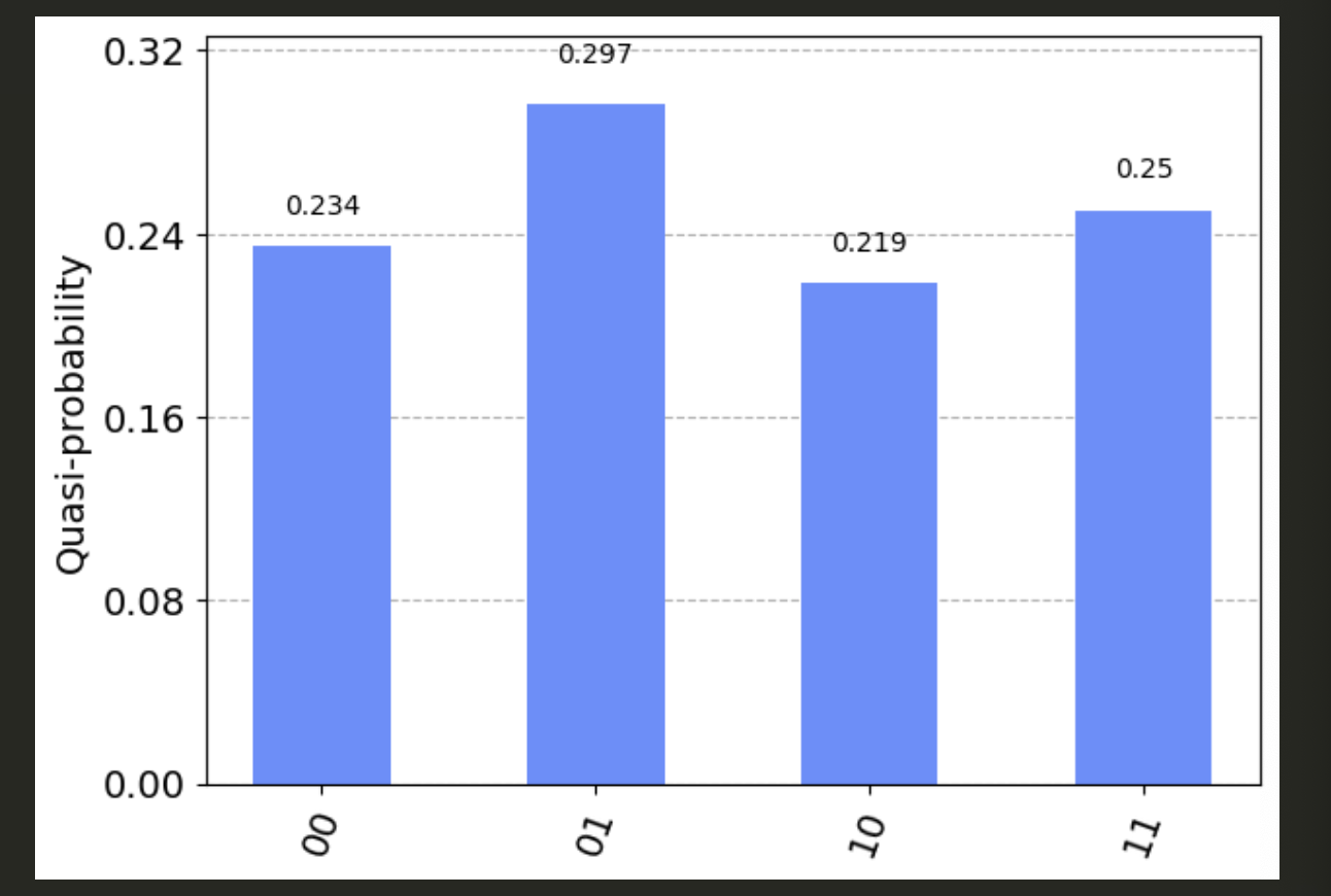
The results show that each computational basis state has approximately equal probability (1/4). The measurement outputs are now defined as classical bits.
Let’s apply the same circuit (excluding measurement gates) to the standard computational basis states to observe the outcomes.
# Generating the same circuit, but without the measurement gates
circuit = QuantumCircuit(2)
circuit.h(0)
circuit.cx(0, 1)
circuit.cz(1, 0)
circuit.h(1)
circuit.cz(0, 1)

zero, one = Statevector.from_label("0"), Statevector.from_label("1")

standard_basis_states = [zero.tensor(zero), zero.tensor(one),
                         one.tensor(zero), one.tensor(one)]
names = ["|00>", "|01>", "|10>", "|11>"]

for i in range(len(standard_basis_states)):
    print(f"{names[i]} -->")
    display(standard_basis_states[i].evolve(circuit).draw("latex"))
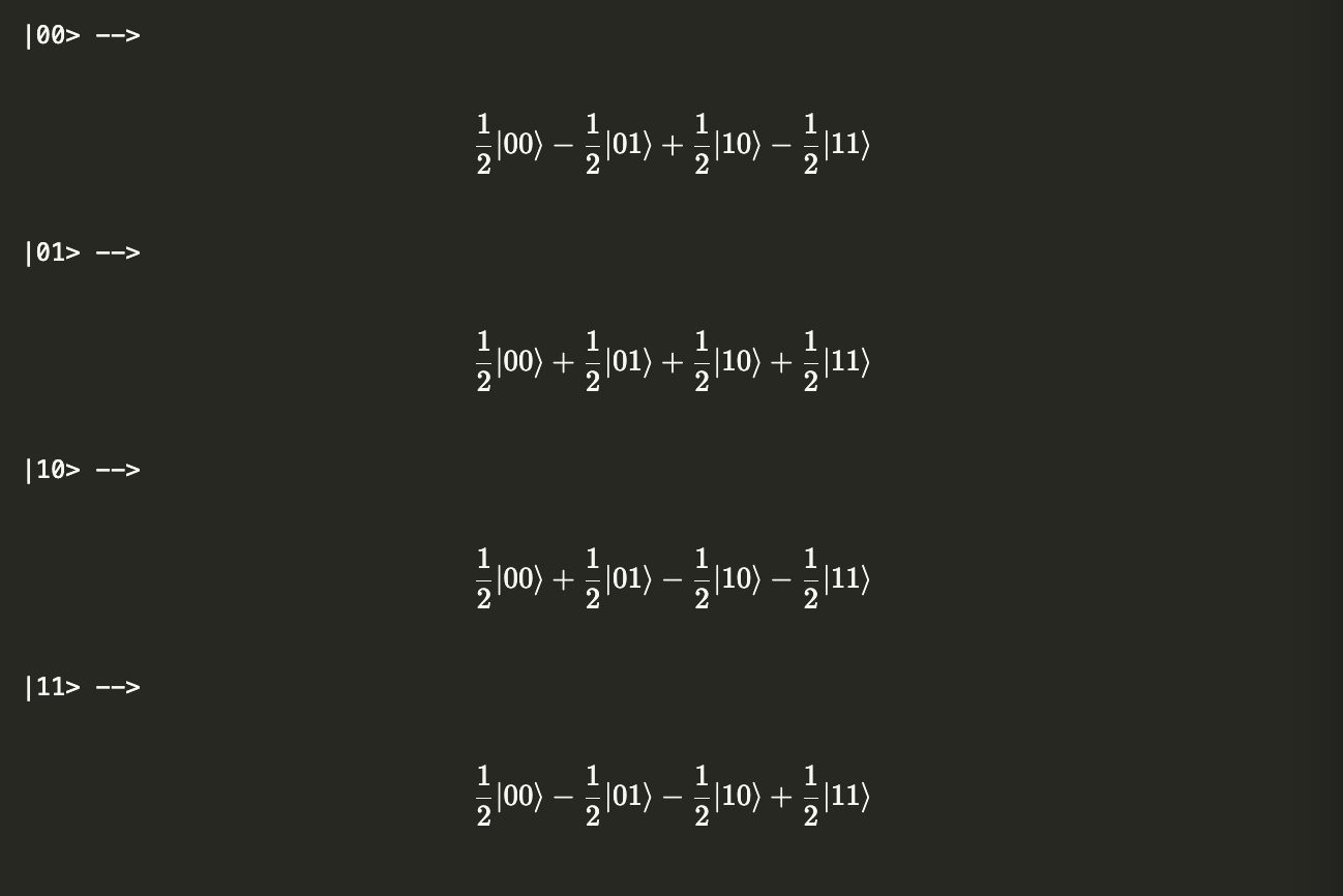
Each state has an equal probability of 1/4.
Now, let’s apply the circuit to a more complex state vector.
plus = Statevector.from_label("+")
vec = Statevector([(1 + 2.0j)/3, -2/3])
statevec = plus.tensor(vec)

statevec.draw('latex')

The post-circuit statevector:
display(statevec.evolve(circuit).draw('latex'))

After applying the circuit, the possible measurement outcomes are only $|00\rangle$ or $|11\rangle$.
This differs from the sampler results above because the sampler runs on the defined quantum circuit, which initializes all the qubits to $|0\rangle$. In contrast, we ran the circuit on a more complex statevector, leading to different possible measurement outcomes.
Exercises
- Generate the following circuit using the diagram below.

Implement the circuit from Problem 1 on the statevector given by $|+-+-\rangle$. What is the resultant statevector? Plot the probability distributions for 4000 samples using
plot_histogram().Add a measurement gate to all the qubits using the
circuit.measure_all()method. You should yield the following circuit:

Afterwards use a sampler primitive to visualize the classical probabilities resulting from this circuit. What are the possible classical results?
$\hspace{1px}$
$\hspace{1px}$
$\hspace{1px}$
$\hspace{1px}$
$\hspace{1px}$
$\hspace{1px}$
Solutions
Problem 1.
from qiskit import QuantumCircuit

circuit = QuantumCircuit(4)

circuit.h(range(4)) # Applying Hadamard on all four Qubits
circuit.cx(2, 3)
circuit.cx(3, 1)
circuit.h(range(3))

circuit.draw()

Problem 2.
Let’s first generate the statevector for $|+-+-\rangle$. To do this I first generate the tensor product $|+\rangle |-\rangle$. I then take its tensor product with itself to yield $|+\rangle|-\rangle|+\rangle|-\rangle = |+-+-\rangle$.
from qiskit.quantum_info import Statevector

plus = Statevector.from_label('+')
minus = Statevector.from_label('-')

plusminus = plus.tensor(minus) # Generating |+>|->
plusminus_twice = plusminus.tensor(plusminus) # Generating |+>|->|+>|-> = |+-+->

plusminus_twice.draw("latex")

Applying the circuit from Problem 1,
plusminus_twice.evolve(circuit).draw('latex')

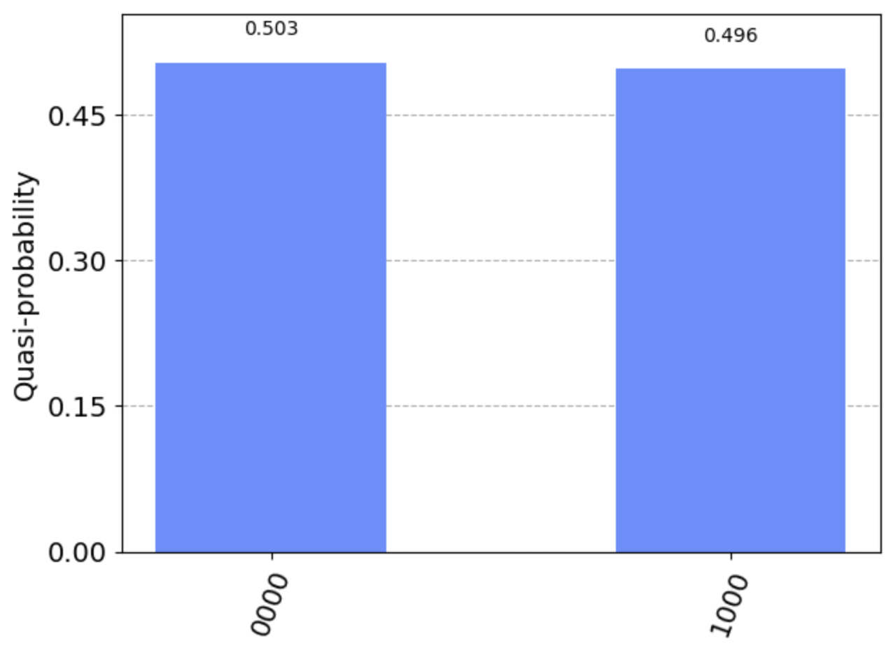
We don’t really need to plot a histogram of the probabilities for each eigenvector – we can see clearly they are all 1/8th. But let’s do it anyways for practice.
from qiskit.visualization import plot_histogram

results = plusminus_twice.evolve(circuit).sample_counts(4000)
plot_histogram(results)
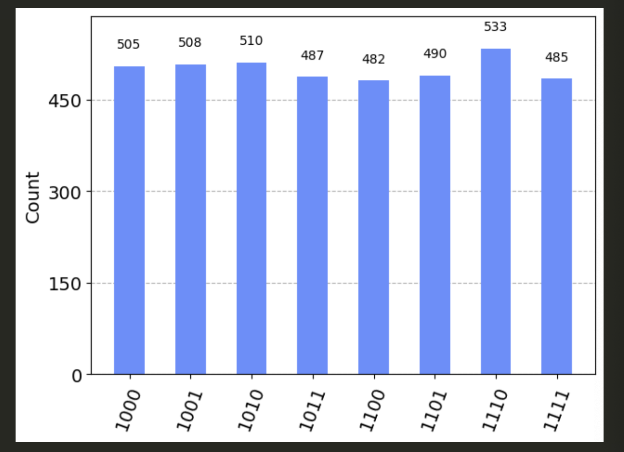
From 4000 sample runs we get a rough 500 yields for each state – a 1/8th probability.
Problem 3
Let’s add the measurement gates to the circuit from Problem 1 using measure_all()
circuit = QuantumCircuit(4)

circuit.h(range(4)) # Applying Hadamard on all four Qubits
circuit.cx(2, 3)
circuit.cx(3, 1)
circuit.h(range(3))

# ---- same as problem 1 thus far ---- #

circuit.measure_all() # Apply a measurement gate on all four Qubits
                      # Stores the results as classical bits
                      # Notice how we did not specify any classical wire
                      # Calling .measure() automatically produced appropriate
                      # classical wires to store the results

circuit.draw()

Notice the rectangular barrier that was automatically placed to separate the measurement gates from the quantum circuit. This circuit.barrier() is used for visualization and aesthetic purposes.
Let’s use the sampler primitive to visualize the probabilities resulting from this circuit.
from qiskit.primitives import Sampler

sampler = Sampler() # initilialize Sampler
job = sampler.run(circuit, shots = 4000) # 4000 samples
results = job.result()

statistics = results.quasi_dists[0].binary_probabilities()

plot_histogram(statistics)
Previous – Multi-Qubit States $\sim$*$\backsim$ Next – Quantum Teleportation
