$$ \sim * \backsim $$
Table of Contents
- § 9. Quantum Entanglement
- § 10. Entanglement as a resource
- § 11. Teleportation
- § 12. Teleportation using Qiskit
- Exercises
- Solutions
$$ \backsim * \sim $$
By this point, you should have a good understanding of Qiskit as a language. We know how to define any n-qubit state and build a circuit to operate on it.
The chapters will now start to contain more information outside of purely code cells. We are moving directly into quantum computing theory.
§ 9. Quantum Entanglement
I will provide a quick lesson on understanding quantum entanglement. For those who already know, skip to the next section.
Suppose that $|\phi\rangle$ is a quantum statevector of a system $X$ and $|\psi\rangle$ is a quantum statevector of a system $Y$. The tensor product $|\phi\psi\rangle = |\phi\rangle \otimes |\psi\rangle$ is a valid quantum statevector of the joint system $(X, Y)$. We refer to a state of this form as a product state—a state that can be simplified to a tensor product of two other states.
Intuitively, when a pair $(X, Y)$ is in a product state $|\phi\rangle \otimes |\psi\rangle$, we can interpret this as $X$ being in the state $|\phi\rangle$ and $Y$ being in the state $|\psi\rangle$. The states are independent of each other; they simply exist in a joint system $(X, Y)$.
However, not all statevectors of multiple systems are product states (i.e., they cannot be reduced to a tensor product of other statevectors). For example, consider the following Bell state:
$$\frac{1}{\sqrt{2}}|00\rangle + \frac{1}{\sqrt{2}}|11\rangle$$
This is not a product state. If it were, there would exist statevectors $|\phi\rangle$ and $|\psi\rangle$ such that
$$|\phi\rangle \otimes |\psi\rangle = \frac{1}{\sqrt{2}}|00\rangle + \frac{1}{\sqrt{2}}|11\rangle$$
However, if this were the case, it would mean that
$$ \langle 0 |\phi\rangle \langle 1 | \psi \rangle = \langle 01 | \phi \otimes \psi \rangle = 0$$
(since there is no $|01\rangle$ component). This implies that either $\langle 0 | \phi\rangle = 0$ or $\langle 1 | \psi \rangle = 0$ (or both). But if this were the case,
$$ \langle 0 |\phi \rangle \langle 0 | \psi \rangle = \langle 00 | \phi \otimes \psi \rangle = \frac{1}{\sqrt{2}}$$
and
$$ \langle 1 |\phi \rangle \langle 1 | \psi \rangle = \langle 11 | \phi \otimes \psi \rangle = \frac{1}{\sqrt{2}}$$
would not both be able to be nonzero. It follows that the Bell state represents a correlation between two systems – we call this entanglement.
§ 10. Entanglement as a resource
Recall the bell state $|\phi^+\rangle$, an entangled quantum state given by
$$|\phi^+\rangle = \frac{1}{\sqrt{2}}|00\rangle + \frac{1}{\sqrt{2}}|11\rangle \qquad \qquad (1)$$
Let’s also consider the following probabilistic 2-qubit state:
$$\frac{1}{2}|00\rangle + \frac{1}{2}|11\rangle \qquad \qquad \qquad \qquad \quad (2)$$
In some sense, (2) is similar to the Bell state, though it is not normalized. It represents a probabilistic state in which the two qubits are correlated. However, since it is not normalized (not a valid quantum state), we do not regard (2) as entangled. Entanglement is a uniquely quantum phenomenon.
Entanglement is usually described in one of two ways:
-
If one of two entangled qubits is measured, then the state of the other qubit is somehow instantaneously affected.
-
The state of the two qubits together cannot be described separately; the qubits somehow maintain a memory of each other.
These statements are true for entangled states, but why are they not true for the un-entangled state (2)? The two bits represented in (2) are intimately connected: each one has a perfect memory of the other in a literal sense. Nevertheless, it is not an entangled state.
This chapter will explain what makes the quantum state (1) very different from the probabilistic state (2). Specifically, we’ll explore what can be done with entanglement that cannot be achieved with any classically correlated state like (2).
For terminology, we refer to entangled states like (1) as an e-bit. Even though (1) consists of two qubits, due to entanglement, we can represent it as one e-bit.
§ 11. Teleportation
Quantum teleportation is a protocol where a sender (Alice) sends a qubit to a receiver (Bob) using a shared entangled quantum state (one e-bit) and two bits of classical information. The term teleportation does not refer to quantum tunneling or the teleportation of matter. Instead, what is teleported is quantum information.
Here is the setup for teleportation:
We assume Alice and Bob share an e-bit: Alice holds qubit $A$, Bob holds qubit $B$, and together the pair ($A, B$) is in the state $|\phi^+\rangle$, as given by (1). For example, Alice and Bob might have been in the same location in the past, where they prepared qubits $A$ and $B$ in the state $|\phi^+\rangle$, and then separated with one qubit each.
Alice then comes into possession of a third qubit $Q$ that she wishes to send to Bob. The state of qubit $Q$ is considered to be unknown to both Alice and Bob, with no assumptions made. $Q$ could even be entangled with other systems that Alice and Bob have no knowledge of.
In the context of teleportation, Alice cannot physically send qubit $Q$ to Bob. However, she can send classical information to him. This is practical since we know how to send classical information over long distances via the internet.
No one knows how to transmit a qubit over a long distance (without its wave function de-localizing). But everyone knows how to send classical information via the web.
You might wonder why we need an e-bit at all. Is it possible to communicate quantum information using only classical communication? The answer is no. To understand why, let’s discuss the no-cloning theorem.
No-Cloning Theorem
The no-cloning theorem shows that it is impossible to create a perfect copy of an unknown quantum state.
Let $X$ and $Y$ be systems sharing the same classical state set $\Sigma$. (Could be the computational basis {${|0\rangle, |1\rangle}$}, but doesn’t have to be). There does not exist a quantum state $|\phi\rangle$ of $Y$ and a unitary operation $U$ on the pair $(X, Y)$ such that $U(|\psi\rangle \otimes |\phi\rangle) = |\psi\rangle \otimes |\psi\rangle$ for every state $|\psi\rangle$ of $X$.
In other words, there is no way to initialize the system $Y$ (to any state $|\phi\rangle$) and perform a unitary operation $U$ on the joint system $(X, Y)$, such that the state $|\psi\rangle$ is cloned—resulting in $(X, Y)$ being in the state $|\psi\rangle \otimes |\psi\rangle$.
Proof
Let’s assume there exists a quantum state $|\phi\rangle$ of $Y$ and a unitary operation $U$ on the pair $(X, Y)$, such that $U(|\psi\rangle \otimes |\phi\rangle) = |\psi\rangle \otimes |\psi\rangle$ for every quantum state $|\psi\rangle$ of $X$.
Then it would be the case that:
$$U(|a\rangle \otimes |\phi\rangle) = |a\rangle \otimes |b\rangle \qquad \text{and} \qquad U(|b\rangle \otimes |\phi\rangle) = |b\rangle \otimes |b\rangle$$
However, a property of the tensor product is that it is linear. Therefore, we must also have:
$$U \left( \left( \frac{1}{\sqrt{2}}|a\rangle + \frac{1}{\sqrt{2}} |b\rangle \right) \otimes |\phi\rangle \right) = \frac{1}{\sqrt{2}}|a\rangle \otimes |a\rangle + \frac{1}{\sqrt{2}}|b\rangle \otimes |b\rangle.$$
But the requirement that $U(|\psi \rangle \otimes |\phi\rangle) = |\psi\rangle \otimes |\psi\rangle$ for every state $|\psi\rangle$ demands that:
$$ \begin{aligned} U &\left( \left( \frac{1}{\sqrt{2}}|a\rangle + \frac{1}{\sqrt{2}} |b\rangle \right) \otimes |\phi\rangle \right) \\ &= \left( \frac{1}{\sqrt{2}} |a\rangle + \frac{1}{\sqrt{2}} |b\rangle \right)\otimes \left( \frac{1}{\sqrt{2}} |a\rangle + \frac{1}{\sqrt{2}}|b\rangle\right) \\ &= \frac{1}{2}|a\rangle \otimes |a\rangle + \frac{1}{2}|a\rangle \otimes |b\rangle + \frac{1}{2}|b\rangle \otimes |a\rangle + \frac{1}{2}|b\rangle \otimes |b\rangle \\ &\neq \frac{1}{\sqrt{2}} |a\rangle \otimes |a\rangle + \frac{1}{\sqrt{2}}|b\rangle \otimes |b\rangle. \end{aligned} $$
Therefore, there can’t exist a state $|\phi\rangle$ and a unitary operation $U$ for which $U(|\psi\rangle \otimes |\phi\rangle) = |\psi\rangle \otimes |\psi\rangle$ for every quantum state vector $|\psi\rangle$. Perfect cloning is impossible, though there are ways to clone with limited accuracy—which we won’t get into here.
This should give you some intuition as to why it is impossible to communicate quantum information using classical communication alone. Any classical transmission from Alice to Bob might also potentially be received by a second receiver (call him Charlie). But if Charlie receives the same information that Bob received, would he not also be able to obtain a copy of the qubit $Q$? This would suggest $Q$ was cloned—which we know is impossible from the no-cloning theorem.
However, when the assumption that Alice and Bob share an e-bit is in place, it is possible for Alice and Bob to accomplish their task. This is known as the quantum teleportation protocol.
Protocol
Here is the quantum circuit diagram that describes the teleportation protocol:
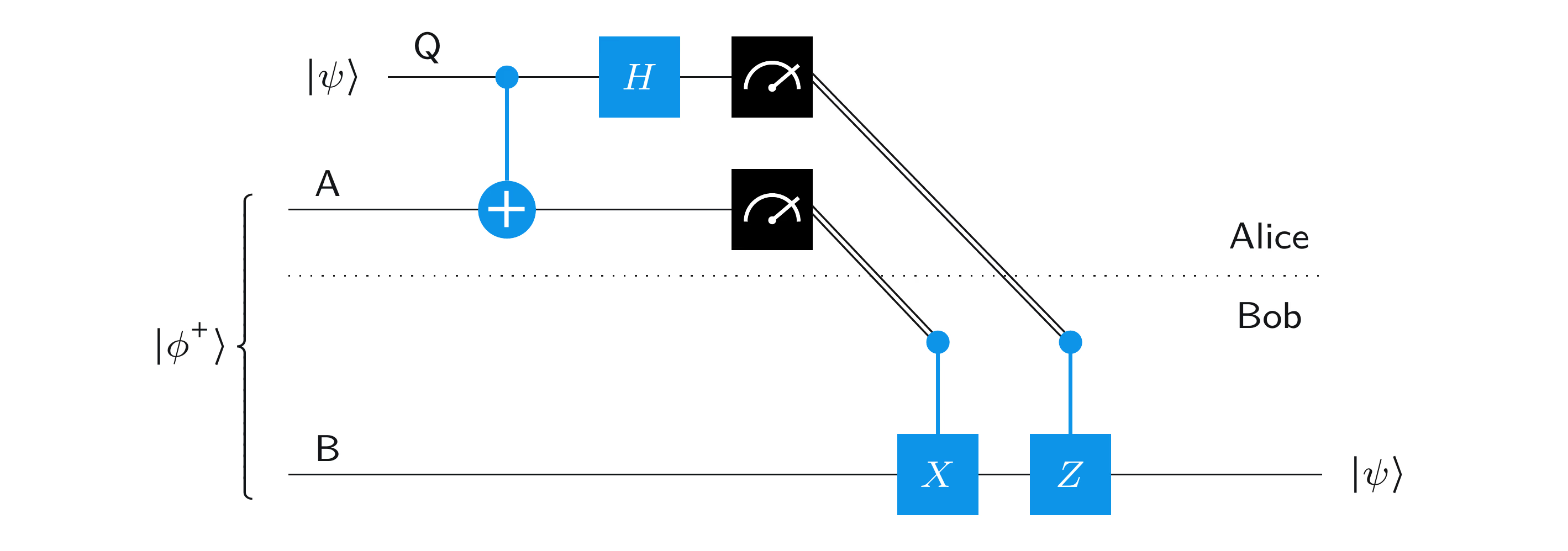 Figure 8: Teleportation Protocol
Retrieved from IBM Quantum Learning
The upper half of the circuit diagram is essentially the inverse of the circuit we used to construct the Bell basis from the computational basis at the beginning of chapter 3. The protocol is as follows:
-
Alice performs a CNOT operation on the pair ($A, Q$), with $Q$ as the control and $A$ as the target. She then performs a Hadamard gate on $Q$.
-
Alice measures both $A$ and $Q$ using standard basis measurement gates and transmits the classical outcomes to Bob. Let’s call the outcome of measuring $A$ as $a$ and the outcome of measuring $Q$ as $b$.
-
Bob receives $a$ and $b$ from Alice. Depending on the values of these bits, he performs the following operations:
- if $a=1$, Bob performs a bit-flip ($X$ gate) on his qubit $B$.
- if $b=1$, Bob performs a phase-flip ($Z$ gate) on his qubit $B$
| (ab) | Operation |
|---|---|
| 00 | Identity |
| 01 | Z |
| 10 | X |
| 11 | ZX |
After these operations, $B$ will be in the same state that $Q$ was in before the protocol was executed, including any correlations it had with other systems. This means the protocol has effectively created a perfect qubit communication channel, where the state of $Q$ has been teleported into $B$.
This protocol does not succeed in cloning the state of $Q$, which we know is impossible. Instead, the state of the qubit $Q$ becomes $|b\rangle$ after being measured. The e-bit also gets destroyed as $A$ becomes $|a\rangle$, losing its entanglement with $B$. Let’s actually do the math behind how teleportation works.
Analysis
Let’s analyze the circuit described above, one step at a time. Beginning with the situation in which $Q$ is some arbitrary state $\underline{\alpha|0\rangle + \beta|1\rangle}$. This does not capture the possibility of $Q$ being entangled with other systems, but let’s start with it for now.
Let’s consider the states of the qubits $(B, A, Q)$ at the times suggested by the figure:
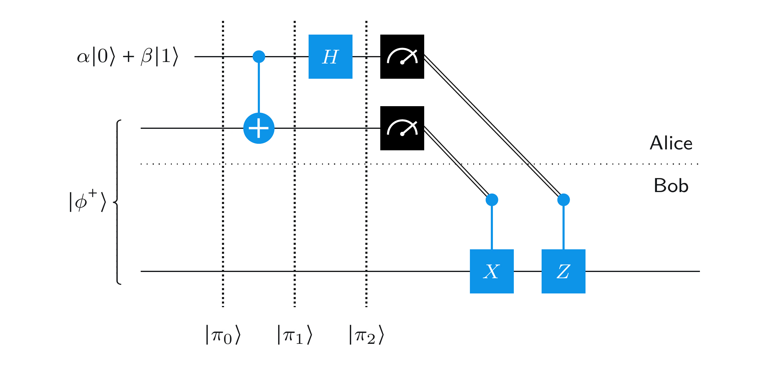 Figure 9: Three $|\pi\rangle$ states to analyze
Retrieved from IBM Quantum Learning
Note this analysis is directly from IBM Quantum Learning (with a bit of improvement in clarity and explanation). I am providing the information here as well so you don’t have to go back and forth.
The state of the three qubits ($B, A, Q$) together at the start of the protocol is
Starting State $|\pi_0\rangle$
$$ \begin{aligned} |\pi_0\rangle &= |B\rangle \otimes |A\rangle \otimes |Q\rangle \\ &= |\phi^+\rangle \otimes (\alpha|0\rangle + \beta|1\rangle) = \left(\frac{1}{\sqrt{2}}|00\rangle + \frac{1}{\sqrt{2}}|11\rangle \right) \otimes (\alpha|0\rangle + \beta|1\rangle) \\ &= \frac{1}{\sqrt{2}} (\alpha|000\rangle + \alpha|110\rangle + \beta|001\rangle + \beta|111\rangle) \end{aligned} $$
Second State $|\pi_1\rangle$
The first gate that is performed is the CNOT gate, where the $Q$ (third qubit) component is the control, and the $A$ (second qubit) component is the target. Remember we are in the system ($B, A, Q$).
This transforms $|\pi_0\rangle$ into
$$ |\pi_0\rangle = \frac{1}{\sqrt{2}} (\alpha|000\rangle + \alpha|110\rangle + \beta|001\rangle + \beta|111\rangle) $$
$$ \downarrow $$
$$ |\pi_1\rangle = \frac{1}{\sqrt{2}} (\alpha|000\rangle + \alpha|110\rangle + \beta|011\rangle + \beta|101\rangle) $$
when the third qubit $Q$ is 1, the second qubit $A$ bit-flips.
Third State $|\pi_3\rangle$
Afterwards a Hadamard Gate is applied on $Q$, the third qubit. This transforms $|\pi_1\rangle$ into
$$ |\pi_1\rangle = \frac{1}{\sqrt{2}} (\alpha|000\rangle + \alpha|110\rangle + \beta|011\rangle + \beta|101\rangle) $$
$$ \downarrow $$
$$ \begin{align} |\pi_2\rangle &= \frac{1}{\sqrt{2}} (\alpha |00\rangle |+\rangle + \alpha|11\rangle|+\rangle + \beta|01\rangle |-\rangle + \beta|10\rangle|-\rangle) \\ &= \frac{1}{2} (\alpha|000\rangle + \alpha|001\rangle + \alpha|110\rangle + \alpha|111\rangle + \beta|010\rangle - \beta|011\rangle + \beta|100\rangle - \beta|101\rangle) \end{align} $$
This makes sense since the Hadamard Gate turns $|0\rangle \to |+\rangle$ and $|1\rangle \to | - \rangle$. The rest is just algebraic manipulation - expanding $|+\rangle$ and $|-\rangle$ in terms of {$|0\rangle, |1\rangle$} and performing all the tensor products.
Using the multi-linearity of the tensor product, we may alternatively state $|\pi_2\rangle$ as follows:
$$ \begin{align} |\pi_2\rangle &= \frac{1}{2}(\alpha|0\rangle + \beta|1\rangle)|00\rangle \\ &+ \frac{1}{2}(\alpha|0\rangle - \beta|1\rangle)|01\rangle \\ &+ \frac{1}{2}(\alpha|1\rangle + \beta|0\rangle)|10\rangle \\ &+ \frac{1}{2}(\alpha|1\rangle - \beta|0\rangle)|11\rangle \end{align} $$
Check for yourself by expanding this and comparing it to the long version of $|\pi_2\rangle$ above.
Now, the leftmost qubit $B$ has the coefficients $\alpha$ and $\beta$. You might be very confused—how can $B$ depend on $\alpha$ and $\beta$ when there hasn’t been any communication between Alice and Bob yet? This is just an illusion. All we have done is use algebra to express the $|\pi_2\rangle$ state in a way that makes the analysis easier. $\alpha$ and $\beta$ are not specifically associated with the leftmost qubit $B$ any more than they are with the other qubits.
Now let’s consider the four possible outcomes of Alice’s standard basis measurements, along with the gates Bob performs as a result.
Possible Measurement Outcomes
$(ab) = 00$ case
The outcome of Alice’s measurement is $ab = 00$ with probability 1/4. In this case the state ($B, A, Q$) collapses into
$$ (\alpha |0\rangle + \beta|1\rangle)|00\rangle $$
Bob does nothing in this case (identity operation).
This is the final state of these qubits: $$ |BAQ\rangle_{00} =\underline{(\alpha|0\rangle + \beta|1\rangle)}|00\rangle .$$
$(ab) = 01$ case
The outcome of Alice’s measurement is $ab = 01$ with probability 1/4. In this case, the state ($B, A, Q$) collapses into
$$ (\alpha|0\rangle - \beta|1\rangle)|01\rangle$$
Bob then applies a $Z$ gate to qubit $B$. The state ($B, A, Q$) becomes
$$ (\alpha|0\rangle + \beta|1\rangle)|01\rangle $$
This is the final state of these qubits: $$ |BAQ\rangle_{01} =\underline{(\alpha|0\rangle + \beta|1\rangle)}|01\rangle .$$
$(ab) = 10$ case
The outcome of Alice’s measurement is $ab = 10$ with probability 1/4. In this case the state ($B, A, Q$) collapses into
$$ (\alpha|1\rangle + \beta|0\rangle)|10\rangle$$
Bob then applies an $X$ gate to qubit $B$. The state ($B, A, Q$) becomes
$$ (\alpha|0\rangle + \beta |1\rangle)|10\rangle $$
This is the final state of these qubits: $$ |BAQ\rangle_{10} =\underline{(\alpha|0\rangle + \beta|1\rangle)}|10\rangle .$$
$(ab) = 11$ case
The outcome of Alice’s measurement is $ab = 11$ with probability 1/4. In this case the state ($B, A, Q$) collapses into
$$(\alpha|1\rangle -\beta|1\rangle)|11\rangle$$
Bob then performs the operation $ZX$ on qubit $B$. The state ($B, A, Q$) becomes $$(\alpha|0\rangle + \beta|1\rangle)|11\rangle$$
This is the final state of these qubits: $$ |BAQ\rangle_{11} =\underline{(\alpha|0\rangle + \beta|1\rangle)}|11\rangle. $$
As you have probably noticed, in all four cases, Bob’s qubit $B$ is left in the state:
$$|B\rangle = \underline{\alpha|0\rangle + \beta|1\rangle}.$$
This is the same state as $Q$ was originally in. The teleportation protocol worked!
Alice no longer has the state $\alpha|0\rangle + \beta|1\rangle$, in accordance with the no-cloning theorem. Most importantly, Alice’s classical measurements yield absolutely no information about the state $\alpha|0\rangle + \beta|1\rangle$. The probability for each outcome is 1/4, irrespective of $\alpha$ and $\beta$.
General $Q$ case
Let’s consider the general situation in which the qubit $Q$ is initially entangled with another system, which we will name $R$. A similar analysis to the one above reveals that the teleportation protocol functions correctly even in the general case. At the end, the qubit $B$ held by Bob is entangled with $R$ in the same way $Q$ was originally. How is this possible?
Suppose the state of the pair ($Q, R$) is initially given by the quantum state vector of the form
$$ \underline{\alpha|0\rangle_Q |\gamma_0\rangle_R + \beta|1\rangle_Q |\gamma_1\rangle_R }$$
where $|\gamma_0\rangle$ and $|\gamma_1\rangle$ are unit vectors and $\alpha$ and $\beta$ are complex numbers satisfying the normalization condition $|\alpha|^2 + |\beta|^2 = 1$. We implement the same circuit diagram, with the addition of the system $R$, represented by a collection of qubits at the top where nothing happens.
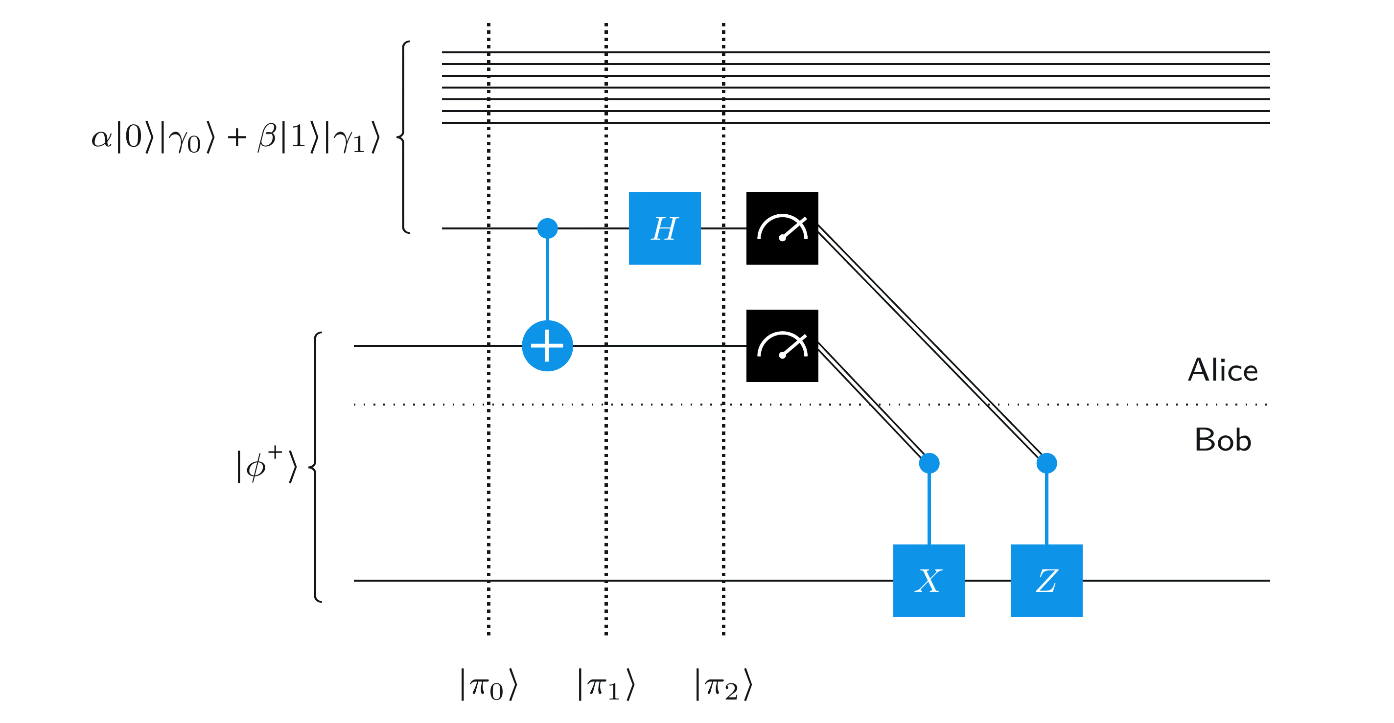 Figure 10: General Q Teleportation Protocol
Retrieved from IBM Quantum Learning
We will consider the state of the system in the order ($B, R, A, Q$). The names of the various systems will be included as subscripts for clarity.
Starting State $|\pi_0\rangle$
At the start of the protocol, the state of the system is as follows:
$$ \begin{align} |\pi_0\rangle &= |\phi^+\rangle_{BA} \otimes (\alpha|0\rangle_Q |\gamma_0\rangle_R + \beta|1\rangle_Q |\gamma_1\rangle_R) \\ &= \frac{1}{\sqrt{2}} (\alpha|0\rangle_B |\gamma_0\rangle_R |00\rangle_{AQ} + \alpha|1\rangle_B |\gamma_0\rangle_R |10\rangle_{AQ} + \beta|0\rangle_B |\gamma_1\rangle_R |01\rangle_{AQ} + \beta|1\rangle_B |\gamma_1\rangle_R |11\rangle_{AQ} \end{align} $$
Second State $|\pi_1\rangle$
First the CNOT gate is applied, with qubit $Q$ as the control and $A$ as the target. This transforms the state into $|\pi_1\rangle$:
$$ |\pi_1\rangle = \frac{1}{\sqrt{2}} (\alpha|0\rangle_B |\gamma_0\rangle_R |00\rangle_{AQ} + \alpha|1\rangle_B |\gamma_0\rangle_R |10\rangle_{AQ} + \beta|0\rangle_B |\gamma_1\rangle_R |11\rangle_{AQ} + \beta|1\rangle_B |\gamma_1\rangle_R |01\rangle_{AQ} $$
Second State $|\pi_2\rangle$
Then the Hadamard Gate is applied. Post-tensor product and algebraic simplification, we get
$$ \begin{align} |\pi_2\rangle &= \frac{1}{2}(\alpha|0\rangle_B |\gamma_0\rangle_R + \beta|1\rangle_B |\gamma_1\rangle_R |00\rangle_{AQ}) \\ &= \frac{1}{2}(\alpha|0\rangle_B |\gamma_0\rangle_R - \beta|1\rangle_B |\gamma_1\rangle_R |01\rangle_{AQ}) \\ &= \frac{1}{2}(\alpha|1\rangle_B |\gamma_0\rangle_R + \beta|0\rangle_B |\gamma_1\rangle_R |10\rangle_{AQ}) \\ &= \frac{1}{2}(\alpha|1\rangle_B |\gamma_0\rangle_R + \beta|0\rangle_B |\gamma_1\rangle_R |11\rangle_{AQ}) \end{align} $$
Just like before, let’s consider the four possible outcomes of Alice’s standard basis measurements, along with the gates Bob performs as a result.
Possible Measurement Outcomes
The probabilities for yielding $|00\rangle_{AQ}$ to $|11\rangle_{AQ}$ are all 1/4. Again, let’s consider the classical result of measuring qubit $A$ to be $a$, and the result of measuring qubit $Q$ to be $b$.
$(ab) = 00$ case
If $(ab) = 00$, the state $|\pi_2\rangle$ collapses into
$$ (\underline{\alpha|0\rangle_B |\gamma_0\rangle_R) + \beta|1\rangle_B |\gamma_1\rangle_R})|00\rangle_{AQ} $$
We do nothing to this state since $a, b$ are both 0. This is the final state for this case.
$(ab) = 01$ case
If $(ab) = 01$, the state $|\pi_2\rangle$ collapses into
$$ (\alpha|0\rangle_B |\gamma_0\rangle_R - \beta|1\rangle_B |\gamma_1\rangle_R)|01\rangle_{AQ} $$
Since $b = 1$, we perform a $Z$ (-1 phase-flip) gate to qubit $B$. This transforms the state into
$$ (\underline{\alpha|0\rangle_B |\gamma_0\rangle_R + \beta|1\rangle_B |\gamma_1\rangle_R})|01\rangle_{AQ} $$
This is the final state for this case.
$(ab) = 10$ case
If $(ab) = 10$, the state $|\pi_2\rangle$ collapses into
$$ (\alpha|1\rangle_B |\gamma_0\rangle_R + \beta|0\rangle_B |\gamma_1\rangle_R)|10\rangle_{AQ}$$
Since $a = 1$, we perform a $X$ (bit-flip) operation on qubit $B$. This transforms the state into
$$ (\underline{\alpha|0\rangle_B |\gamma_0\rangle_R + \beta|1\rangle_B |\gamma_1\rangle_R})|10\rangle_{AQ} $$
$(ab) = 11$ case
If $(ab) = 11$, the state $|\pi_2\rangle$ collapses into
$$ (\alpha|1\rangle_B |\gamma_0\rangle_R - \beta|0\rangle_B |\gamma_1\rangle_R)|11\rangle_{AQ}$$
Since both $a, b = 1$, we perform a $ZX$ (-1 phase flip & bit-flip) operation on qubit $B$. This transforms the state into
$$ (\underline{\alpha|0\rangle_B |\gamma_0\rangle_R + \beta|1\rangle_B |\gamma_1\rangle_R})|11\rangle_{AQ} $$
We find that at the end of the protocol, the state of $(B, R)$ is always
$$ \underline{\alpha|0\rangle_B|\gamma_0\rangle_R + \beta|1\rangle_B|\gamma_1\rangle_R} $$
which is the initial entangled state between $Q$ and $R$. Except this time, the entanglement is between $B$ and $R$.
Isn’t that cool? The math makes sense, but it’s mind-blowing how it works. Just by transmitting classical information, you can recreate a state that is automatically entangled with another state you don’t even know about. Quantum mechanics is crazy weird but also incredibly fascinating! Teleportation succeeds in creating a perfect quantum communication channel.
Since this protocol creates a perfect copy of any arbitrary state, entangled or not, it must reduce to the identity matrix. I won’t present a proper proof of this yet (probably for a while), but if you are interested in the math, look it up!
Teleportation might become the way to communicate quantum information, just like how we use bits for classical communication today. The future quantum web might be full of CNOT and Hadamard gates. (Probably not exactly, but who knows!)
Let’s finally code the teleportation circuit using Qiskit!
§ 12. Teleportation using Qiskit
Let’s first import the necessary QuantumCircuit() imports.
from qiskit import QuantumCircuit, QuantumRegister, ClassicalRegister
from qiskit_aer import AerSimulator
from qiskit.visualization import plot_histogram
from qiskit.result import marginal_distribution
from qiskit.circuit.library import UGate
from numpy import pi, random
Note – you may get an import error saying imported module qiskit_aer not found. This is because qiskit_aer is a separate installation from Qiskit. Run pip install qiskit_aer and ensure you are using the python kernel where it gets installed.
If all is in order…let’s continue. The following code generates the teleportation protocol we spent an hour learning about.
qubit = QuantumRegister(1, "Q")
ebit0 = QuantumRegister(1, "A")
ebit1 = QuantumRegister(1, "B") #ebit0 and ebit1 will be entangled
a = ClassicalRegister(1, "a")
b = ClassicalRegister(1, "b")
protocol = QuantumCircuit(qubit, ebit0, ebit1, a, b)
# Entangles qubits A and B into the |Φ+> state.
# Bell circuit from the beginning of Chapter 3.
protocol.h(ebit0)
protocol.cx(ebit0, ebit1)
protocol.barrier() # aesthetic barrier
# Alice's operations
protocol.cx(qubit, ebit0)
protocol.h(qubit)
protocol.barrier()
# Alice's measurements, placing the results in classical bits
# `a` and `b` for Bob
protocol.measure(ebit0, a)
protocol.measure(qubit, b)
protocol.barrier()
# Bob uses classical results from `a` and `b` to conditionally
# apply gates
with protocol.if_test((a, 1)):
protocol.x(ebit1)
with protocol.if_test((b, 1)):
protocol.z(ebit1)
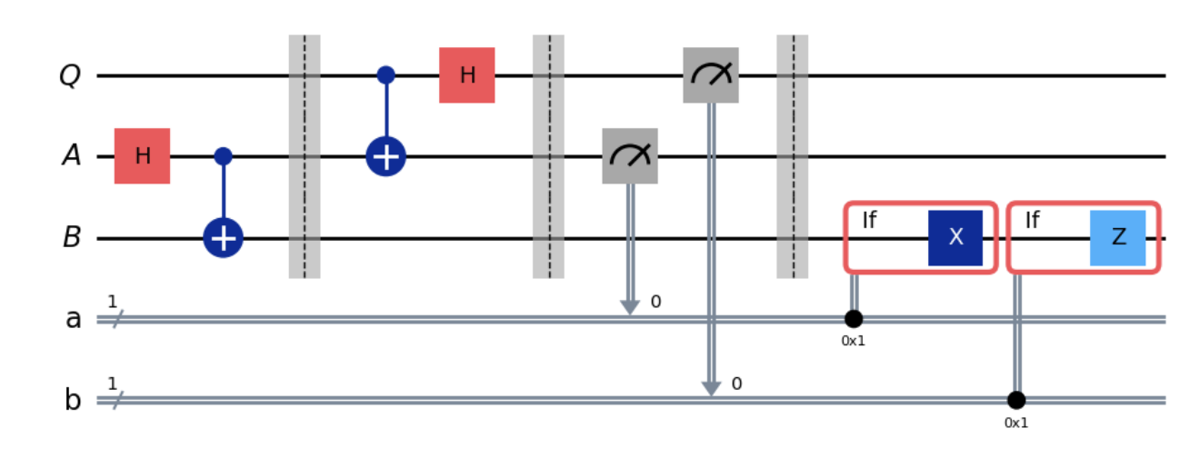
protocol.draw('mpl')
Before we proceed further, it’s crucial to have a solid understanding of the code we’ve discussed. While it’s ideal if you can try building it yourself based on what we’ve learned, simply comprehending it is a good start. I’ll test your understanding later.
The circuit we’re discussing includes the barrier() function I mentioned earlier, along with if_test functions, which essentially check if a condition a == 1 is met.
The circuit first initializes $(A, B)$ to be in the $|\phi^+\rangle$ state. This entanglement step is crucial for the protocol but isn’t part of the actual teleportation protocol.
Testing Teleportation
Even though the math works you probably are still confused and skeptical. Me too. Let’s actually test that the protocol we programmed works.
To validate our protocol, let’s apply a randomly generated single-qubit gate to the initialized $|0\rangle$ state of $Q$, creating a randomized statevector $Q$. This new randomized state is the state we aim to teleport into $B$.
After running the protocol, we’ll reverse the random gate applied to $B$. If $B$ returns to the $|0\rangle$ state, it confirms that the protocol has worked together, meaning $B$ held the randomized $Q$.
Now, let’s proceed to generate the random unitary gate needed to randomize $Q$.
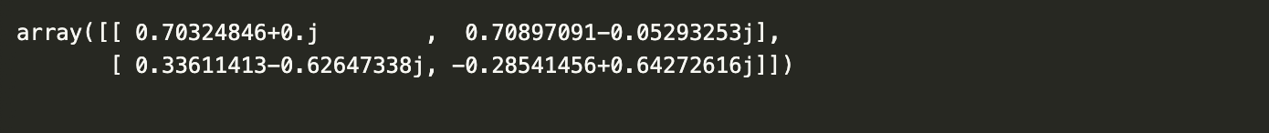
random_gate = UGate(
    theta = random.random() * 2 * pi,
    phi = random.random() * 2 * pi,
    lam = random.random() * 2 * pi
)

display(random_gate.to_matrix())
Here was my output, yours is most certainly different:
Now we’ll create a new testing circuit that first applies our random gate to $Q$. It then runs the teleportation circuit and afterwards applies the inverse of our randomized unitary gate to the qubit $B$ and measures it. The outcome should be $|0\rangle$.
# Create a new circuit including the same bits and qubits used in the
# teleportation protocol.

test = QuantumCircuit(qubit, ebit0, ebit1, a, b)

# Start with the randomly selected gate on Q

test.append(random_gate, qubit)
test.barrier()

# Append the entire teleportation protocol from above.

test = test.compose(protocol)
test.barrier()

# Finally, apply the inverse of the random unitary to B and measure.

test.append(random_gate.inverse(), ebit1)

result = ClassicalRegister(1, "Result")
test.add_register(result)
test.measure(ebit1, result)

test.draw('mpl')
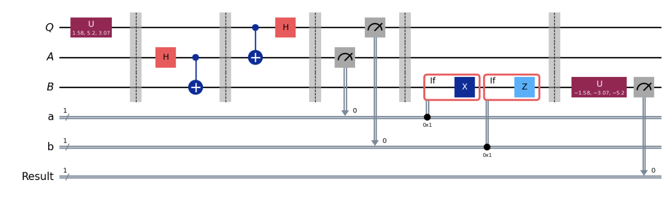
Make sure you understand the circuit, with the additions we made.
Finally, let’s run the AerSimulator() function on the circuit and plot a histogram of the outputs. The AerSimulator() simulates the circuit.
Qiskit Aer as a whole is a “high-performance quantum computing simulator with realistic noise models.” We’ll use it to see if the circuit/protocol works or not.
The histogram will show us the statistics for all three classical bits. The bottom/leftmost bit should always be 0 – indicating $Q$ was successfully teleported into $B$.
result = AerSimulator().run(test).result()
statistics = result.get_counts()
plot_histogram(statistics)
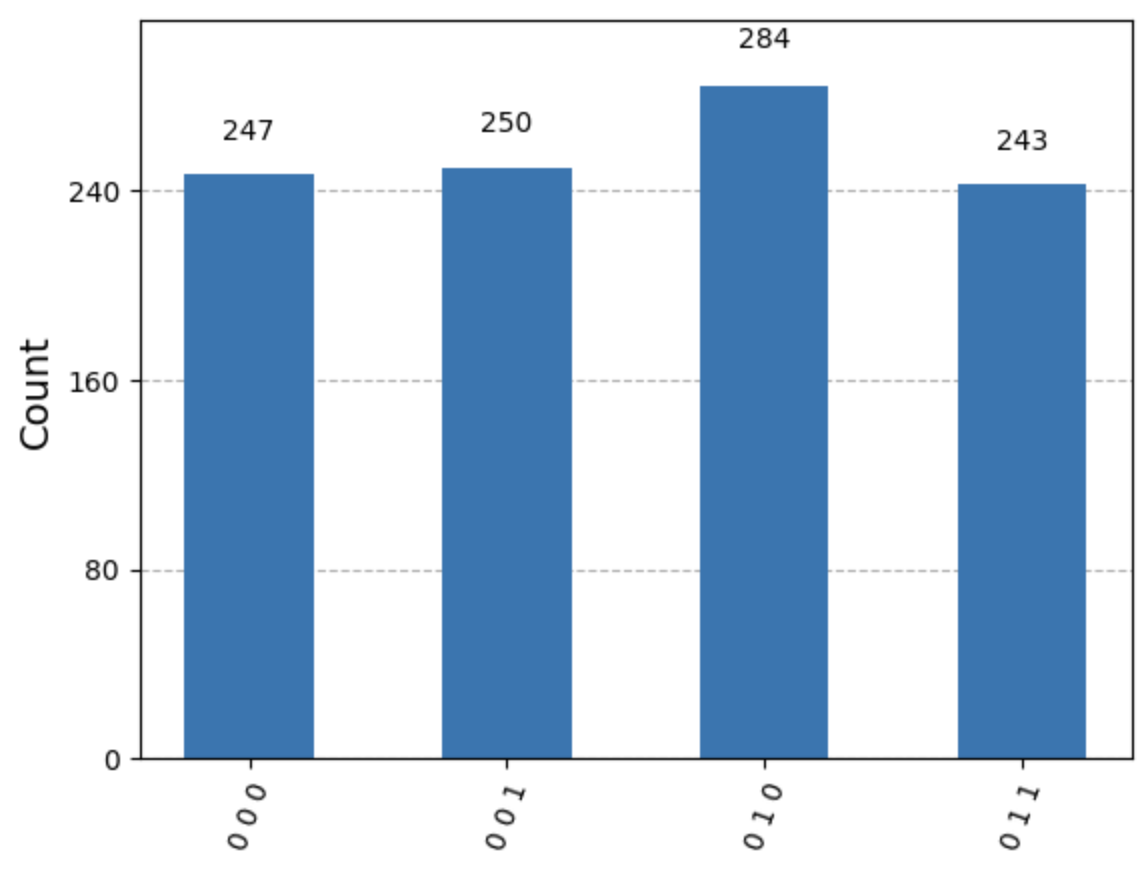
Your bars may look a little different than mine. What is important is that the bottom/leftmost qubit is always 0. This shows the protocol worked.
We can also filter the statistics to focus on just the qubit we want. The bottom/leftmost qubit is, by Qiskit convention, index 2.
filtered_statistics = marginal_distribution(statistics, [2]) # only 2nd index qubit
plot_histogram(filtered_statistics)
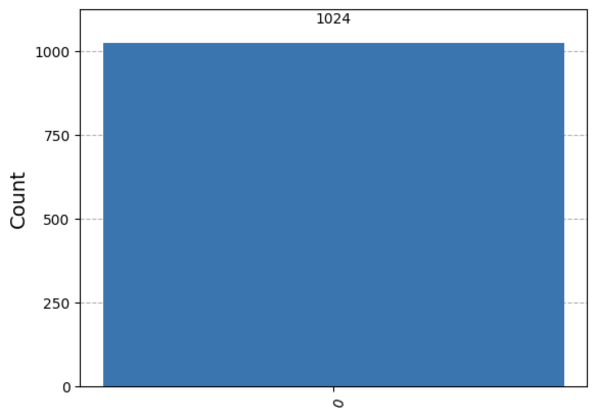
The teleportation protocol worked.
Exercises
Build the $|\phi^+\rangle$ state via the Bell circuit using a Hadamard and CNOT gate. Then, place two measurement gates to map the measurement results of both qubits onto two separate classical bits. Finally, run
AerSimulator()and display a histogram of the results. What are the two classical result possibilities? What are their respective probabilities?Initialize a 2-qubit custom-named circuit. Apply a randomized unitary gate using
UGate()toq_0, the qubit of index 0. Afterwards add the Bell circuit and measurement gates from problem 1. Finally, runAerSimulator()and display a histogram of the results.$\hspace{1px}$
$\hspace{1px}$
$\hspace{1px}$
$\hspace{1px}$
$\hspace{1px}$
$\hspace{1px}$
Solutions
Problem 1.
The Bell circuit is generated as follows:
from qiskit import QuantumCircuit, QuantumRegister, ClassicalRegister
from qiskit.quantum_info import Statevector
from qiskit_aer import AerSimulator
from qiskit.visualization import plot_histogram
from qiskit.result import marginal_distribution
from qiskit.circuit.library import UGate
from numpy import pi, random

qubits = QuantumRegister(2, "qubit")

bell_circuit = QuantumCircuit(qubits) # only including qubits right now

bell_circuit.h(0)
bell_circuit.cx(0, 1)

bell_circuit.draw('mpl')
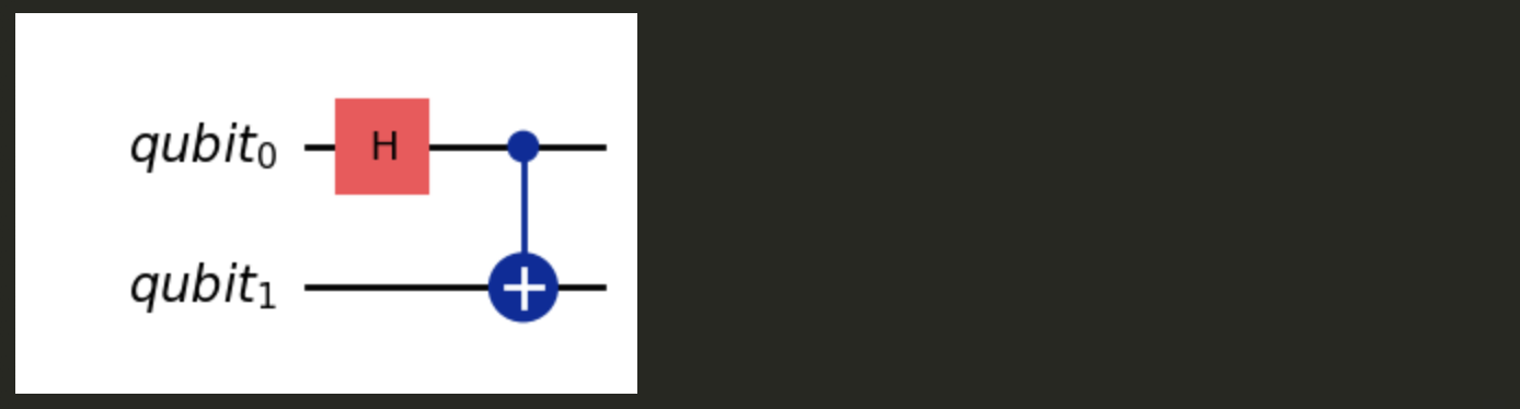
Both qubits in QuantumCircuit() are initialized by default to $|0\rangle$ state. Thus the 2-qubit state we begin with is $|00\rangle$. Applying the bell circuit defined above transforms $|00\rangle \rightarrow |\phi^+\rangle$
zerozero = Statevector.from_label("0").tensor(Statevector.from_label("0"))

zerozero.evolve(bell_circuit).draw("latex")

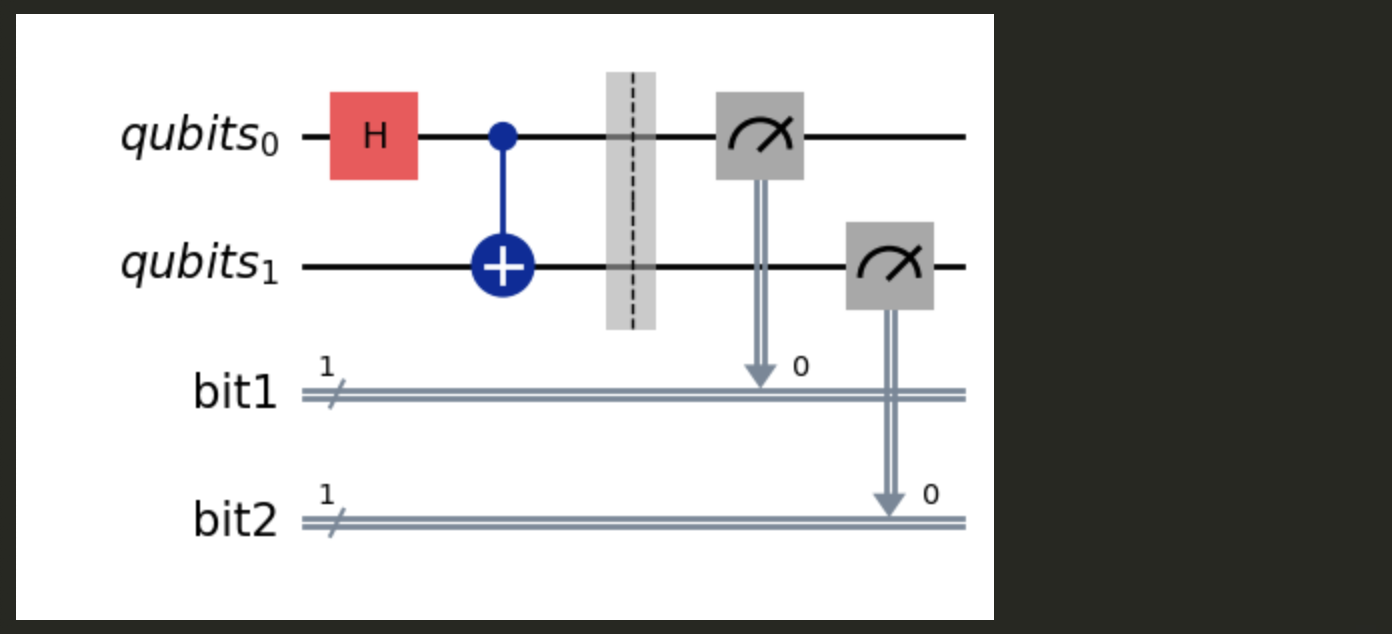
Now let’s add the measurement gates to map the measurement results of both qubits onto two separate classical bits.
bit1 = ClassicalRegister(1, "bit1") # Creating the classical bits
bit2 = ClassicalRegister(1, "bit2")

circuit = QuantumCircuit(qubits, bit1, bit2)
circuit = circuit.compose(bell_circuit) # appending the Bell Circuit to the new
										# initialized circuit
circuit.barrier()

circuit.measure(qubits[0], bit1)
circuit.measure(qubits[1], bit2)

circuit.draw('mpl')
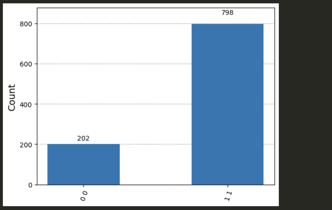
Let’s run AerSimulator() and display a histogram of the measurement results
job = AerSimulator().run(circuit, shots = 1000) # 1000 samples
results = job.result()
statistics = results.get_counts()

plot_histogram(statistics)
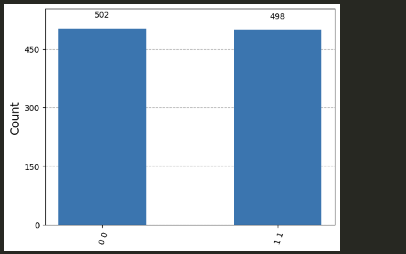
We see a perfect 50/50 probabilitiy of yielding the classical measurements
00 or 11. This is expected from the $|\phi^+\rangle$ state.
Problem 2.
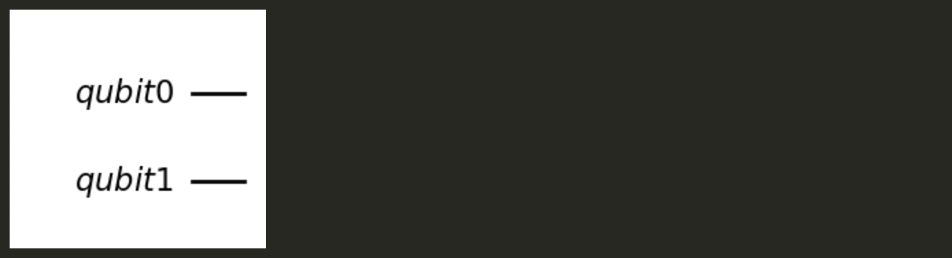
We initialize a 2-qubit custom-named circuit as follows:
qubit0 = QuantumRegister(1, "qubit0")
qubit1 = QuantumRegister(1, "qubit1")

circuit = QuantumCircuit(qubit0, qubit1)
circuit.draw('mpl')
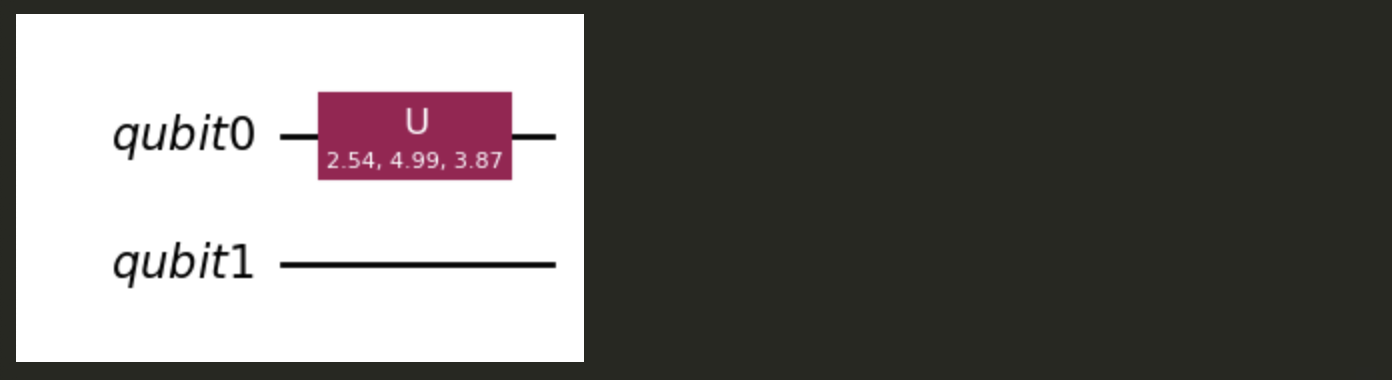
Now let’s generate a random unitary gate using UGate() and apply it to qubit0.
random_gate = UGate(
    theta = random.random() * 2 * pi,
    phi = random.random() * 2 * pi,
    lam = random.random() * 2 * pi
)

random_gate.to_matrix()

circuit.append(random_gate, qubit0)
circuit.draw('mpl')
Let’s add the Bell circuit and measurement gates from Problem 1.
bit0 = ClassicalRegister(1, "bit0")
bit1 = ClassicalRegister(1, "bit1")
bits = QuantumCircuit(bit0, bit1) # Initializing Empty Circuit with 2 Bits


circuit = circuit.compose(bell_circuit) # Adding the Bell Circuit
circuit = circuit.compose(bits) # Adding the two bits to measure onto
circuit.barrier()

circuit.measure(qubit0, bit0)
circuit.measure(qubit1, bit1)


circuit.draw('mpl')
Now let’s run AerSimulator() and display a histogram of the results.
job = AerSimulator().run(circuit, shots = 1000) # 1000 samples
results = job.result()
statistics = results.get_counts()

plot_histogram(statistics)
If I generate a different unitary gate and re-run the AerSimulator(),
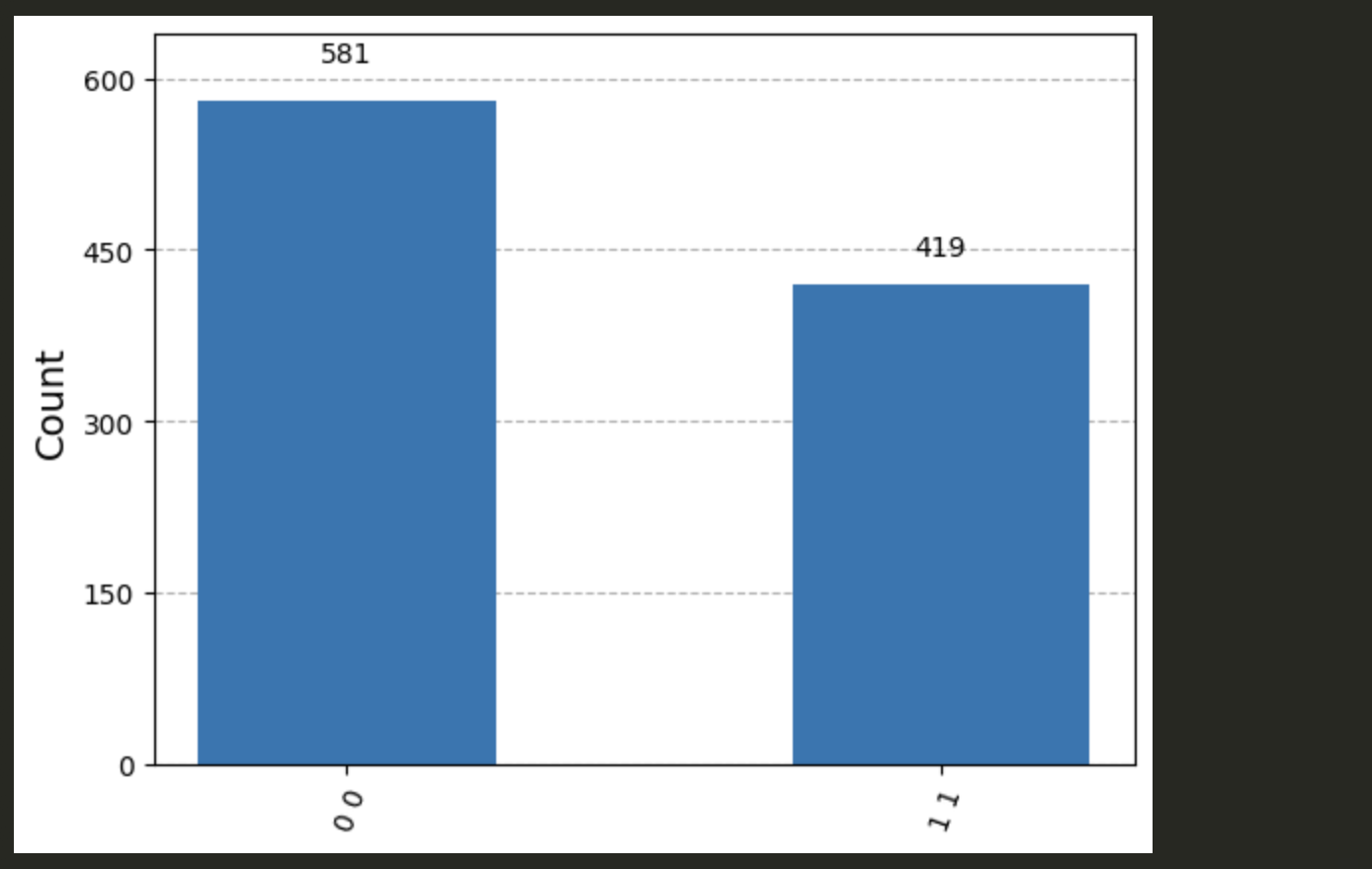
I get something completely different!
Previous – Quantum Circuits $\sim$*$\backsim$ Next – Superdense Coding