Let’s start performing some data analysis with our beautiful JWST near-infrared catalogs. But first! let’s go over what color-magnitude diagrams (CMDs) are. CMDs are the life and blood for astronomers. If you are familiar with the Hertzsprung Russell (HR) diagram, CMDs are a subset of these plots.
They are actually fairly simple. You merely take magnitudes of stars from one catalog ($y$) and plot it relative to the difference in magnitudes between two different catalogs ($x$). An example for both F115W vs. (F115W - F212N) and F212N vs. (F115W - F212N) is shown below.
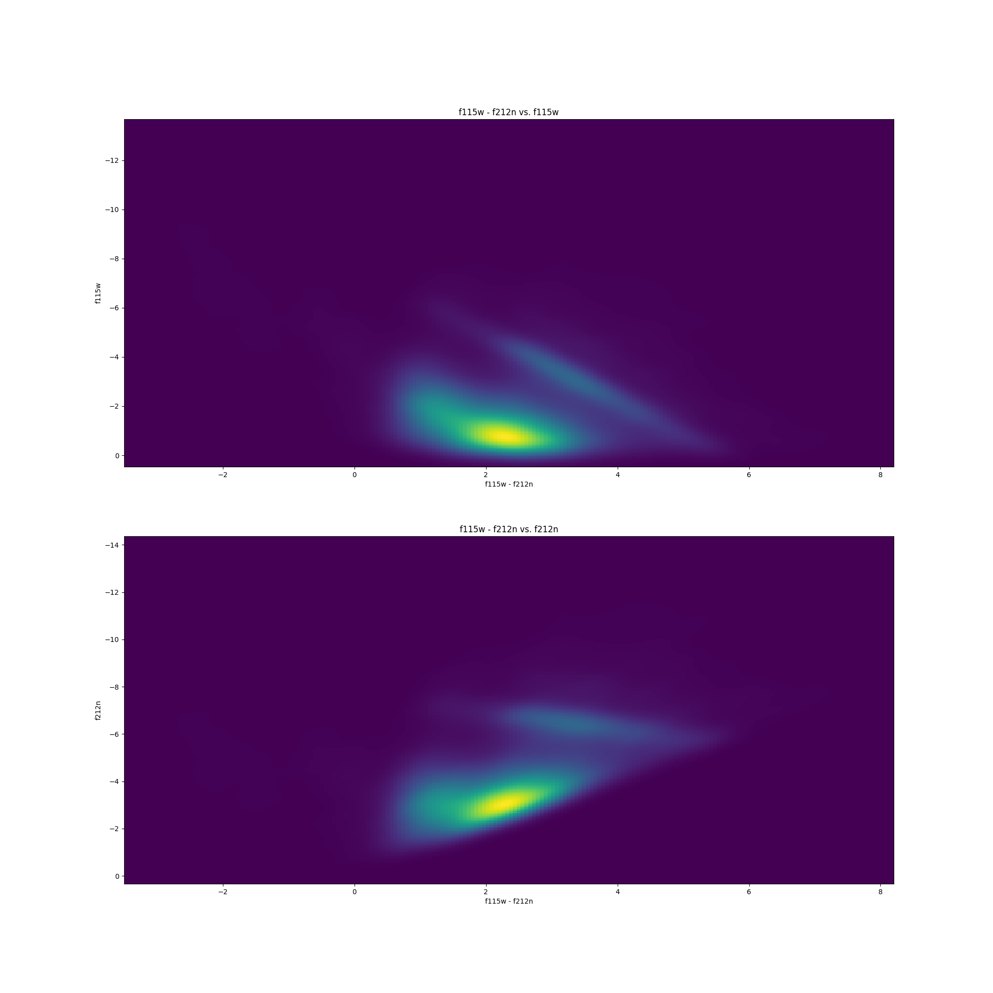
It is standardized to plot the (smaller $\lambda$ - larger $\lambda$) on the $x$-axis.
Now without getting into too much detail, different types of stars occupy different regions of the CMD. The large dense cluster of stars in the plots above showcase the main-sequence track of the CMD, and the linear streak above the main-sequence cluster contains the Red Clump (RC) stars – which are the stars I will be using in my research.
Let’s actually build the above CMDs for the F115W and F212N catalogs. As the catalogs are of different size, with a vastly different # of stars, we first have to determine which stars are common to both catalogs.
As the catalogs are close in wavelength and were taken at approximately the same time, we can assume these catalogs place the star’s $x$ and $y$ coordinates on the same coordinate system. Indeed, if we overplot both the F212N and F115W catalog centroid coordinates on top of each other, with an very zoomed in image in the background…
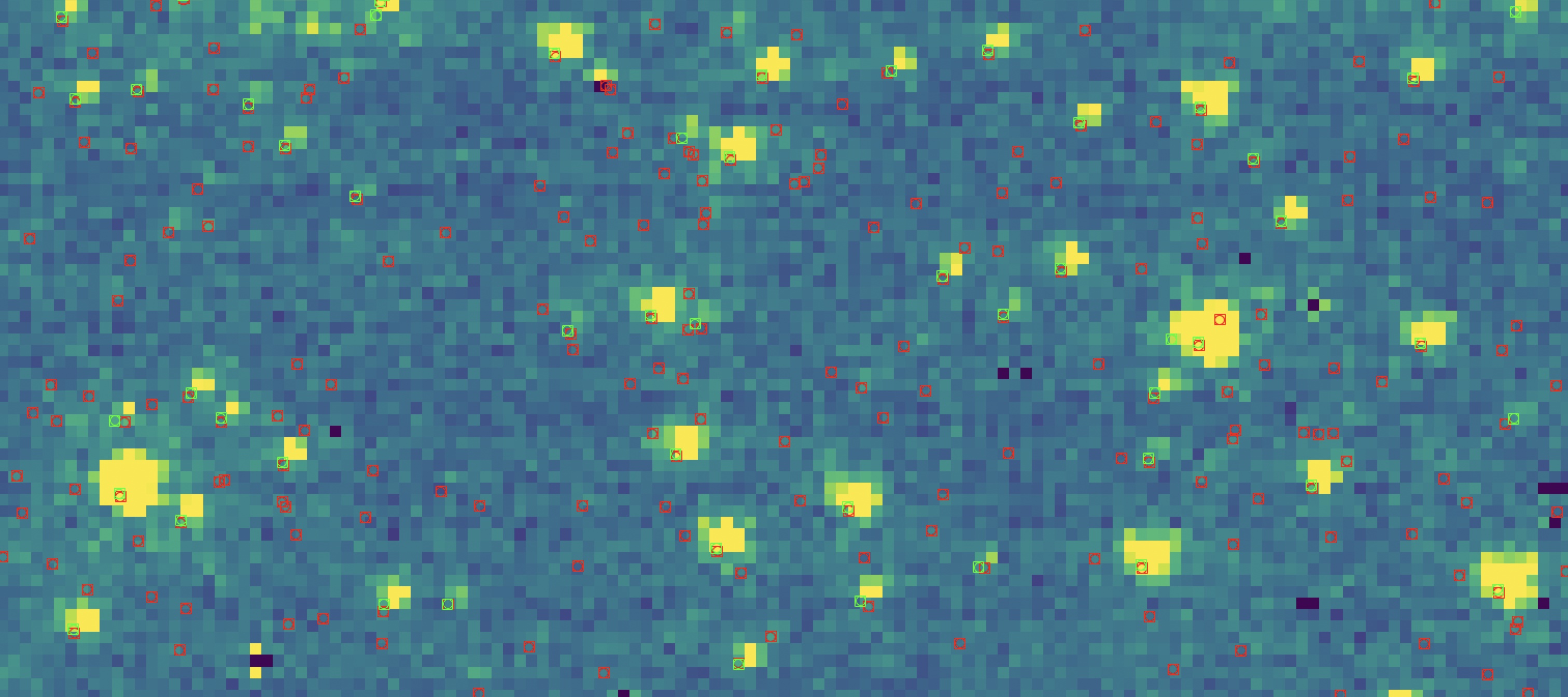
Here, the red squares indicate stars from the F212N catalog, and the green squares indicate stars from the F115W catalog.
As there are 121349 F212N
stars but only 53620 F115W stars for this image, there are a lot more red
markers than green. However, if you look closely you can see for the very
luminous stars, the green and red markers exist on top of one another. Indeed,
the two catalogs are on roughly the same coordinate system. (Note* for future work,
I do perform coordinate transformations on all my catalogs…this is
preliminary work).
Finally, with all the introductions out of the way, we can start doing some research.
Finding Common Stars Across F115W & F212N
To determine the stars common to both F115w and F212n, I employ a nearest-neighbor KDTree algorithm.
No transformations are done and it is assumed that the two catalogs are already on the same coordinate system and magnitude system.
For two stars to be matched, they must be within a specified radius (dr_tol) and
delta-magnitude (dm_tol). For stars with more than 1 neighbor (within the tolerances),
if one is found that is the best match in both brightness and positional offsets
(closest in both), then the match is made. Otherwise,
their is a conflict and no match is returned for the star.
The entire code is shown on my GitHub, but I will lay out some here.
I first start by making coordinate pairs for each star in both catalogs:
if x1.shape != y1.shape:
    raise ValueError('x1 and y1 do not match!')
if x2.shape != y2.shape:
    raise ValueError('x2 and y2 do not match!')

# Setup coords1 pairs and coords 2 pairs
# this is equivalent to, but faster than just doing np.array([x1, y1])
coords1 = np.empty((x1.size, 2))
coords1[:, 0] = x1
coords1[:, 1] = y1

# this is equivalent to, but faster than just doing np.array([x1, y1])
coords2 = np.empty((x2.size, 2))
coords2[:, 0] = x2
coords2[:, 1] = y2
I then implement a KDTree using scipy.spatial
kdt = KDT(coords2, balanced_tree=False)

# This returns the number of neighbors within the specified
# radius. We will use this to find those stars that have no or one
# match and deal with them easily. The more complicated conflict
# cases will be dealt with afterward.
i2_match = kdt.query_ball_point(coords1, dr_tol)
Nmatch = np.array([len(idxs) for idxs in i2_match])
Afterwards, I loop through and handle all the different matches within dr_tol
and dm_tol and place the indices of each star in NumPy Arrays idxs1 and idxs2,
for the first and second catalogs respectively. I then deal with duplicates
# Deal with duplicates
duplicates = [item for item, count in list(Counter(idxs2).items()) if count > 1]
if verbose > 2:
    print(( '    Found {0:d} duplicates out of {1:d} matches'.format(len(duplicates), len(dm))))
keep = np.ones(len(idxs1), dtype=bool)
for dd in range(len(duplicates)):
    # Index into the idxs1, idxs2 array of this duplicate.
    dups = np.where(idxs2 == duplicates[dd])[0]

    # Assume the duplicates are confused first... see if we
    # can resolve the confusion below.
    keep[dups] = False

    dm_dups = m1[idxs1[dups]] - m2[idxs2[dups]]
    dr_dups = np.hypot(x1[idxs1[dups]] - x2[idxs2[dups]], y1[idxs1[dups]] - y2[idxs2[dups]])

    dm_min = np.abs(dm_dups).argmin()
    dr_min = np.abs(dr_dups).argmin()

    # If there is a clearly preferred match (closest in distance and brightness), then
    # keep it and dump the other duplicates.
    if dm_min == dr_min:
        keep[dups[dm_min]] = True
    else:
          if verbose:
              print('confused, dropping')

# Clean up the duplicates
idxs1 = idxs1[keep]
idxs2 = idxs2[keep]
I use the above algorithm with the F115w and F212n catalogs, with a dr_tol of
0.5 and a dm_tol of 99 (I don’t care about dm_tol right now).
And since the algorithm returns the indices of matched stars from their
respective catalogs, I can get the magnitudes for the matched stars by just
taking the values from the m column when the index is in idxs1 or idxs2.
x1 = df['x']        # x centroid position of catalog1 stars
y1 = df['y']        # y centroid position of catalog1 stars
m1 = df['m']        # vega magnitude of catalog1 stars
me1 = df['me']      # error in vega magnitude of catalog1 stars
x2 = df2['x']
y2 = df2['y']
m2 = df2['m']
me2 = df2['me']

m1_error = []
m2_error = []
m1_matched = []
m2_matched = []
m_difference = []

for i in idxs1:
    m1_error += [me1[i]]
    m1_matched += [m1[i]]
for i in idxs2:
    m2_error += [me2[i]]
    m2_matched += [m2[i]]
And since the CMDs are a plot of a magnitude vs mag-difference, I subtract the
m1_matched and m2_matched NumPy arrays to get the $x$-axis for all the
CMDs.
m_difference = np.subtract(m1_matched, m2_matched)
Now we have everything we need to generate the CMDs for our catalogs. I implement every step above for all the NRCB1 - NRCB4 catalogs for F115W and F212N.
N1_115_catalog = Table.read("catalogs/dr2/NRCB1_catalog115w.csv").to_pandas()
N1_212_catalog = Table.read("catalogs/dr2/NRCB1_catalog212n.csv").to_pandas()
N1_115_matched, N1_212_matched, N1_115_error, N1_212_error, N1_115_212_difference = matched(N1_115_catalog, N1_212_catalog, "NRCB1_F115W", "NRCB1_F212N", 0.5, 99)

N2_115_catalog = Table.read("catalogs/dr2/NRCB2_catalog115w.csv").to_pandas()
N2_212_catalog = Table.read("catalogs/dr2/NRCB2_catalog212n.csv").to_pandas()
N2_115_matched, N2_212_matched, N2_115_error, N2_212_error, N2_115_212_difference = matched(N2_115_catalog, N2_212_catalog, "NRCB2_F115W", "NRCB2_F212N", 0.5, 99)

N3_115_catalog = Table.read("catalogs/dr2/NRCB3_catalog115w.csv").to_pandas()
N3_212_catalog = Table.read("catalogs/dr2/NRCB3_catalog212n.csv").to_pandas()
N3_115_matched, N3_212_matched, N3_115_error, N3_212_error, N3_115_212_difference = matched(N3_115_catalog, N3_212_catalog, "NRCB3_F115W", "NRCB3_F212N", 0.5, 99)

N4_115_catalog = Table.read("catalogs/dr2/NRCB4_catalog115w.csv").to_pandas()
N4_212_catalog = Table.read("catalogs/dr2/NRCB4_catalog212n.csv").to_pandas()
N4_115_matched, N4_212_matched, N4_115_error, N4_212_error, N4_115_212_difference = matched(N4_115_catalog, N4_212_catalog, "NRCB4_F115W", "NRCB4_F212N", 0.5, 99)
Generating the CMDs
fig, axis = plt.subplots(4, 2, figsize = (20, 20))
fig.suptitle(' NRCB1-NRCB4 All Color-Magnitude Diagrams ', fontsize=15)

axis[0,0].invert_yaxis()
axis[0,1].invert_yaxis()
axis[1,0].invert_yaxis()
axis[1,1].invert_yaxis()
axis[2,0].invert_yaxis()
axis[2,1].invert_yaxis()
axis[3,0].invert_yaxis()
axis[3,1].invert_yaxis()

xy = np.vstack([N1_115_212_difference, N1_115_matched])
z = gaussian_kde(xy)(xy)
axis[0,0].scatter(N1_115_212_difference, N1_115_matched, c = z, s = 1)
axis[0,0].set_xlabel('NRCB1 F115W - F212N')
axis[0,0].set_ylabel('NRCB1 F115W')
axis[0,0].set_title('NRCB1 F115W vs. F115W - F212N')
xy = np.vstack([N1_115_212_difference, N1_212_matched])
z = gaussian_kde(xy)(xy)
axis[0,1].scatter(N1_115_212_difference, N1_212_matched, c = z, s = 1)
axis[0,1].set_xlabel('NRCB1 F115W - F212N')
axis[0,1].set_ylabel('NRCB1 F212N')
axis[0,1].set_title('NRCB1 F212N vs. F115W - F212N')

xy = np.vstack([N2_115_212_difference, N2_115_matched])
z = gaussian_kde(xy)(xy)
axis[1,0].scatter(N2_115_212_difference, N2_115_matched, c = z, s = 1)
axis[1,0].set_xlabel('NRCB2 F115W - F212N')
axis[1,0].set_ylabel('NRCB2 F115W')
axis[1,0].set_title('NRCB2 F115W vs. F115W - F212N')
xy = np.vstack([N2_115_212_difference, N2_212_matched])
z = gaussian_kde(xy)(xy)
axis[1,1].scatter(N2_115_212_difference, N2_212_matched, c = z, s = 1)
axis[1,1].set_xlabel('NRCB2 F115W - F212N')
axis[1,1].set_ylabel('NRCB2 F212N')
axis[1,1].set_title('NRCB2 F212N vs. F115W - F212N')

xy = np.vstack([N3_115_212_difference, N3_115_matched])
z = gaussian_kde(xy)(xy)
axis[2,0].scatter(N3_115_212_difference, N3_115_matched, c = z, s = 1)
axis[2,0].set_xlabel('NRCB3 F115W - F212N')
axis[2,0].set_ylabel('NRCB3 F115W')
axis[2,0].set_title('NRCB3 F115W vs. F115W - F212N')
xy = np.vstack([N3_115_212_difference, N3_212_matched])
z = gaussian_kde(xy)(xy)
axis[2,1].scatter(N3_115_212_difference, N3_212_matched, c = z, s = 1)
axis[2,1].set_title('NRCB3 F212N vs. F115W - F212N')
axis[2,1].set_xlabel('NRCB3 F115W - F212N')
axis[2,1].set_ylabel('NRCB3 F212N')

xy = np.vstack([N4_115_212_difference, N4_115_matched])
z = gaussian_kde(xy)(xy)
axis[3,0].scatter(N4_115_212_difference, N4_115_matched, c = z, s = 1)
axis[3,0].set_xlabel('NRCB4 F115W - F212N')
axis[3,0].set_ylabel('NRCB4 F115W')
axis[3,0].set_title('NRCB4 F115W vs. F115W - F212N')
xy = np.vstack([N4_115_212_difference, N4_212_matched])
z = gaussian_kde(xy)(xy)
axis[3,1].scatter(N4_115_212_difference, N4_212_matched, c = z, s = 1)
axis[3,1].set_xlabel('NRCB4 F115W - F212N')
axis[3,1].set_ylabel('NRCB4 F212N')
axis[3,1].set_title('NRCB4 F212N vs. F115W - F212N')
fig.tight_layout()
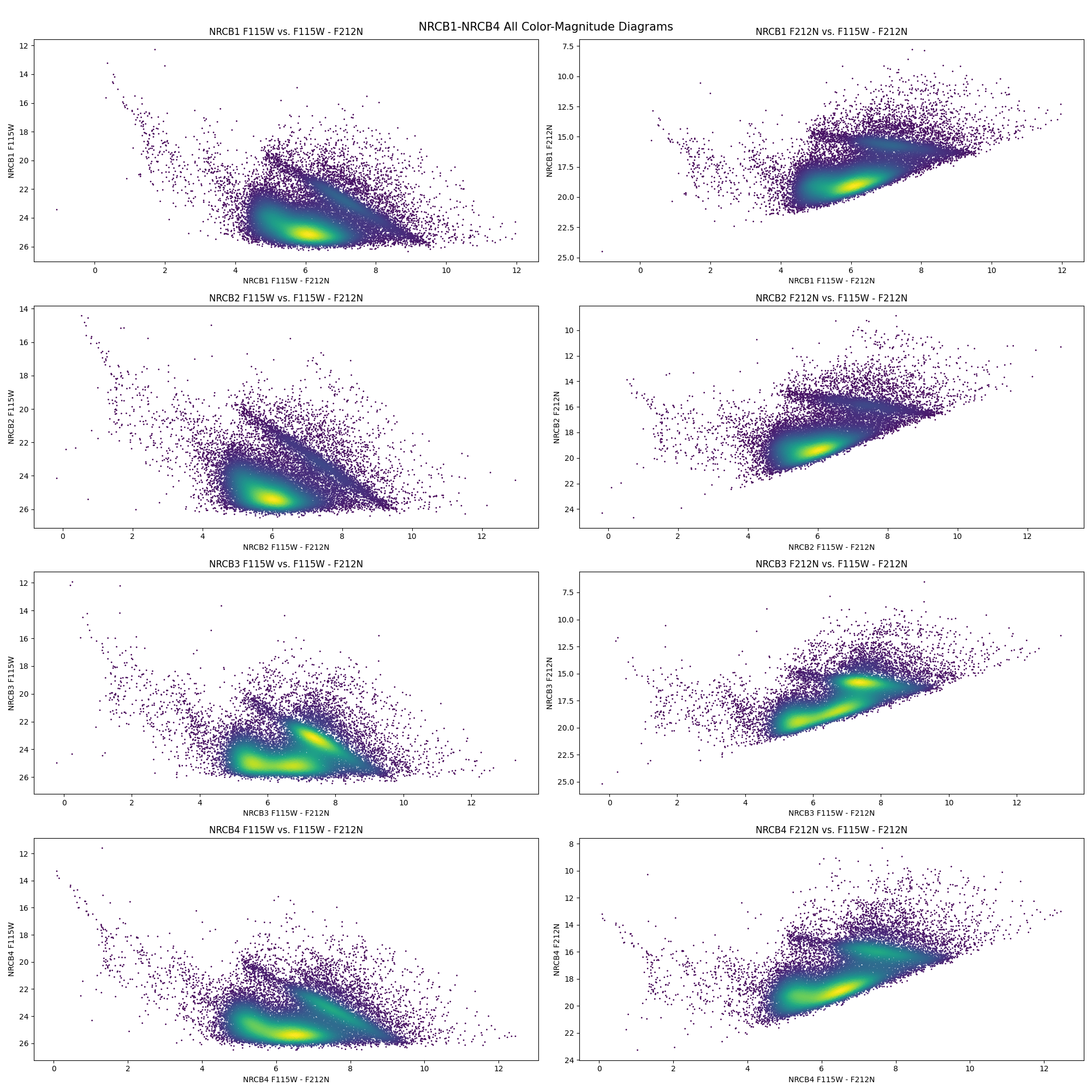
Beautiful! These CMDs have a clear main-sequence track and a very prominent RC bar with a definite slope. The NRCB1 (top row) CMDs match exactly to the CMDs we saw originally. The region NRCB3 is of particular interest since its the region containing Sagittarius A*.
We will now work on seeing how well past extinction laws match the slope of the RC Bar by utilizing theoretical synthetic isochrones for the Galactic Center. Eventually, we’ll derive our own, newer, more accurate extinction laws.